Download
1 / 31
320 likes | 475 Views
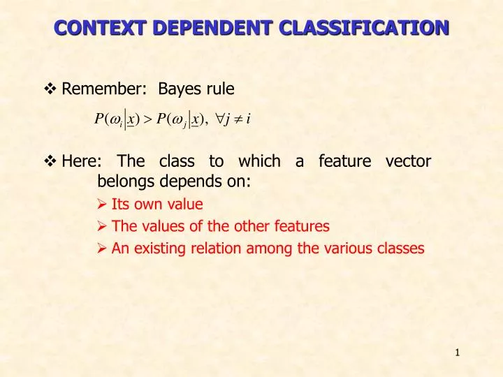
CONTEXT DEPENDENT CLASSIFICATION. Remember: Bayes rule Here: The class to which a feature vector belongs depends on: Its own value The values of the other features An existing relation among the various classes.

E N D
CONTEXT DEPENDENT CLASSIFICATION • Remember: Bayes rule • Here: The class to which a feature vector belongs depends on: • Its own value • The values of the other features • An existing relation among the various classes
This interrelation demands the classification to be performed simultaneously for all available feature vectors • Thus, we will assume that the training vectors occur in sequence, one after the other and we will refer to them as observations
The Context Dependent Bayesian Classifier • Let • Let • Let be a sequence of classes, that is There are MN of those • Thus, the Bayesian rule can equivalently be stated as • Markov Chain Models (for class dependence)
NOW remember: or • Assume: • statistically mutually independent • The pdf in one class independent of the others, then
From the above, the Bayes rule is readily seen to be equivalent to: that is, it rests on • To find the above maximum in brute-force task we need Ο(NMΝ )operations!!
Thus, each Ωi corresponds to one path through the trellis diagram. One of them is the optimum (e.g., black). The classes along the optimal path determine the classes to which ωi are assigned. • To each transition corresponds a cost. For our case
Equivalently where, • Define the cost up to a node ,k,
Bellman’s principle now states • The optimal path terminates at • Complexity O (NM2)
Channel Equalization • The problem
Example • In xk three input symbols are involved: Ik, Ik-1, Ik-2
In this context, ωi are related to states. Given the current state and the transmitted bit, Ik, we determine the next state. The probabilities P(ωi|ωj)define the state dependence model. • The transition cost for all allowable transitions
Assume: • Noise white and Gaussian • A channel impulse response estimate to be available • The states are determined by the values of the binary variables Ik-1,…,Ik-n+1 For n=3, there will be 4 states
Hidden Markov Models • In the channel equalization problem, the states are observable and can be “learned” during the training period • Now we shall assume that states are notobservable and can only be inferred from the training data • Applications: • Speechand Music Recognition • OCR • Blind Equalization • Bioinformatics
An HMM is a stochastic finite state automaton, that generates the observation sequence, x1, x2,…, xN • We assume that: The observation sequence is produced as a result of successive transitions between states, upon arrival at a state:
This type of modeling isused for nonstationarystochastic processes that undergo distinct transitions among a set of different stationary processes.
Examples of HMM: • The single coin case: Assume a coin that is tossed behind a curtain. All it is available to us is the outcome, i.e., H or T. Assume the two states to be: S = 1H S = 2T This is also an example of a random experiment with observable states. The model is characterized by a single parameter, e.g.,P(H). Note that P(1|1) = P(H) P(2|1) = P(T) = 1 – P(H)
The two-coins case: For this case, we observe a sequence of H or T. However, we have no access to know which coin was tossed. Identify one state for each coin. This is an example where states are not observable. H orT can be emitted from either state. The model depends on four parameters. P1(H), P2(H), P(1|1), P(2|2)
The three-coins case example is shown below: • Note that in all previous examples, specifying the model is equivalent to knowing: • The probability of each observation (H,T) to be emitted from each state. • The transition probabilities among states: P(i|j).
A general HMM model is characterized by the following set of parameters • Κ,number of states
That is: • What is the problem in Pattern Recognition • Given Mreference patterns, each described by an HMM, find the parameters, S, for each of them (training) • Given an unknown pattern, find to which one of the M, known patterns, matches best (recognition)
Recognition: Any path method • Assume the M models to be known (M classes). • A sequence of observations,X, is given. • Assume observations to be emissions upon the arrival on successive states • Decide in favor of the model S* (from the M available) according to the Bayes rule for equiprobablepatterns
For each model S there is more than one possible sets of successive state transitions Ωi, each with probability Thus: • For the efficient computation of the above DEFINE Local activity History
Observe that Compute this for each S
Training • The philosophy: Given a training set X, known to belong to the specific model, estimate the unknown parameters of S, so that the output of the model, e.g. to be maximized • This is a ML estimation problem with missing data
Assumption: Data x discrete • Definitions:
The Algorithm: • Initial conditions for all the unknown parameters. • Step 1: From the current estimates of the model parameters reestimate the new model S from
Step 3: Computego to step 2. Otherwise stop • Remarks: • Each iteration improves the model • The algorithm converges to a maximum (local or global) • The algorithm is an implementation of the EM algorithm