Download
1 / 64
640 likes | 783 Views
Section VI Comparing means & analysis of variance. How to display means- Bars ok in simple situations. Presenting means - ANOVA data.

E N D
Presenting means - ANOVA data One can also add “error bars” to these means. In analysis of variance, these error bars are based on the sample size and the pooled standard deviation, SDe. This SDe is the same residual SDe as in regression.
The “Yardstick” is critical yardstick:_________ 1 µm
The “Yardstick” is critical yardstick:_________ 10 meters
Weight loss comparison Diet mean weight loss (lbs) n Pritikin 5.0 20 UCLA GS 9.0 20 mean difference 4.0 Is 4.0 lbs a “big” difference? Compared to what? What is the “yardstick”?
The variation yardstick SD = 1, SEdiff=0.32 , t=12.6, p value < 0.0001
The variation yardstick SD = 5, SEdiff=1.58, t= 2.5, p value = 0.02
Comparing MeansTwo groups – t test (review) Mean differences are “statistically significant” (different beyond chance) relative to their standard error (SEd) ___ ____ t = (Y1 - Y2)= “signal” SEd “noise” _ Yi = mean of group i, SEd =standard error of mean difference t is mean difference in SEd units. As |t| increases, p value gets smaller. Rule of thumb: p < 0.05 when |t| > 2 SEd is the “yardstick” for significance t & p value depend on: a) mean difference b) individual variability = SDs c) sample size (n)
How to compute SEd? SEd depends on n, SD and study design. (example: factorial or repeated measures) For a single mean, if n=sample size _ _____ SEM = SD/n = SD2/n __ __ For a mean difference (Y1 - Y2) The SE of the mean difference, SEd is given by _________________ SEd = [ SD12/n1 + SD22/n2 ] or ________________ SEd = [SEM12 + SEM22] If data is paired (before-after), first compute differences (di=Y2i-Y1i) for each person. For paired: SEd =SD(di)/√n
3 or more groups-analysis of variance (ANOVA) Pooled SDs What if we have many treatment groups, each with its own mean and SD? Group Mean SD sample size (n) __ A Y1 SD1 n1 B Y2 SD2 n2 C Y3 SD3 n3 … __ k Yk SDk nk
The PooledSDethe common yardstick SD2pooled error = SD2e = (n1-1) SD12 + (n2-1) SD22 + … (nk-1) SDk2 (n1-1) + (n2-1) + … (nk-1) ____ so, SDe = = SD2e
ANOVA uses pooledSDe to compute SEd and to compute “post hoc” (post pooling) t statistics and p values. ____________________ SEd = [ SD12/n1 + SD22/n2 ] ____________ = SDe (1/n1) + (1/n2) SD1 and SD2 are replaced by SDe a “common yardstick”. If n1=n2=…=n, then SEd = SDe2/n=constant
Multiplicity & F tests Multiple testing can create “false positives”. We incorrectly declare means are “significantly” different as an artifact of doing many tests even if none of the means are truly different. Imagine we have k=four groups: A, B, C and D. There are six possible mean comparisons: A vs B A vs C A vs D B vs C B vs D C vs D
If we use p < 0.05 as our “significance” criterion, we have a 5% chance of a “false positive” mistake for any one of the six comparisons, assuming that none of the groups are really different from each other. We have a 95% chance of no false positives if none of the groups are really different. So, the chance of a “false positive” in any of the six comparisons is 1 – (0.95)6 = 0.26 or 26%.
To guard against this we first compute the “overall” F statistic and its p value. The overall F statistic compares all the group means to the overall mean (M=overall mean). __ F = ni( Yi – M)2/(k-1) =MSx = between group var (SDp)2MSerrorwithin group var __ __ __ =[n1(Y1 – M)2 + n2(Y2-M)2 + …nk(Yk-M)2]/(k-1) (SDp)2 If “overall” p > 0.05, we stop. Only if the overall p < 0.05 will the pairwise post hoc (post overall) t tests and p values have no more than an overall 5% chance of a “false positive”.
Between group variation need graphic
This criterion was suggested by RA Fisher and is called the Fisher LSD (least significant difference) criterion. It is less conservative (has fewer false negatives) than the very conservative Bonferroni criterion. Bonferroni criterion: if making “m” comparisons, declare significant only if p < 0.05/m. It is an “omnibus” test.
F statistic interpretation F is the ratio of between group variation to (pooled) within group variation. This is why this method is called “analysis of variance” Total variation = Variation between (among) the means (between group) + Pooled variation around each mean (within group) Between group variation Within group variation Total variation F = Between/ Within F ≈ 1 -> not significant (R2=Between variation/Total variation)
One way analysis of variancetime to fall data, k= 4 groups, df= k-1 p value SDe2
Means & SDs in sec (JMP) No model ANOVA model, pooled SDe=10.986 sec Why are SEMs not the same??
Mean comparisons- post hoc t Means not connected by the same letter are significantly different
Multiple comparisons-Tukey’s q As an alternative to Fisher LSD, for pairwise comparisons of “k” means, Tukey computed percentiles for q=(largest mean-smallest mean)/SEd under the null hyp that all means are equal. If mean diff > q SEd is the significance criterion, type I error is ≤ α for all comparisons. q > t > Z One looks up”t” on the q table instead of the t table.
t vs q for α=0.05, large n num means=k t q* 2 1.96 1.96 3 1.96 2.34 4 1.96 2.59 5 1.96 2.73 6 1.96 2.85 * Some tables give q for SE, not SEd, so must multiply q by √2.
Mean comparisons-Tukey Means not connected by the same letter are significantly different
Transformations There are two requirements for the analysis of variance (ANOVA) model. 1. Within any treatment group, the mean should be the middle value. That is, the mean should be about the same as the median. When this is true, the data can usually be reasonably modeled by a Gaussian (“normal”) distribution. 2. The SDs should be similar (variance homogeneity) from group to group. Can plot mean vs median & residual errors to check #1 and mean versus SD to check #2.
What if its not true? Two options: a. Find a transformed scale where it is true. b. Don’t use the usual ANOVA model (use non constant variance ANOVA models or non parametric models). Option “a” is better if possible - more power.
Most common transform is log transformation Usually works for: 1. Radioactive count data 2. Titration data (titers), serial dilution data 3. Cell, bacterial, viral growth, CFUs 4. Steroids & hormones (E2, Testos, …) 5. Power data (decibels, earthquakes) 6. Acidity data (pH), … 7. Cytokines, Liver enzymes (Bilirubin…) In general, log transform works when a multiplicative phenomena is transformed to an additive phenomena.
Compute stats on the log scale & back transform results to original scale for final report. Since log(A)–log(B) =log(A/B), differences on the log scale correspond to ratios on the original scale. Remember 10mean(log data) =geometric mean < arithmetic mean monotone transformation ladder- try these Y2, Y1.5, Y1, Y0.5=√Y, Y0=log(Y), Y-0.5=1/√Y, Y-1=1/Y,Y-1.5, Y-2
Balanced designs - ANOVA exampleBrain Weight data, n=7 x 4 = 28, nc=7 obs/cell
Mean brain weights (gms) in Males and Females with and without dementia A balanced* 2 x 2 (ANOVA) design, nc= 7 obs per cell, n=7 x 4 = 28 obs total Means Cell mean
Brain weight, n=7 x 4 = 28 Difference in marginal sex means (Male – Female) 1327.29 - 1210.79 = 116.50, 116.50/2 = 58.25 Difference in marginal dementia means (Yes – No) 1261.43 - 1276.64 = -15.21, -15.21/2 = -7.61 Difference in cell meandifferences-interaction (1321.14 - 1333.43) – (1201.71 - 1219.86) = 5.86 (1321.14 - 1201.71) – (1333.43 - 1219.86) = 5.86 note: 5.86/(2x2) = 1.46 Parallel (additive) when interaction is zero * balanced = same sample size (nc) in every cell
Brain weight ANOVA MODEL: brain wt = sex, dementia , sex*dementia Class Levels Values sex 2 -1 1 dementia 2 -1 1 n=28 observations, nc=7 per cell Source DF Sum of Squares Mean Square F Value p value Model 3 96686 32228.70 451.05 <.0001 Error 24 1715 71.45 = SD2e C Total 27 98402 R-Square CoeffVar Root MSE Mean brain wt 0.9826 0.666092 8.453=SDe 1269.04 Source DF SS Mean Square F Value p value sex 1 95005.75 95005.75 1329.64 <.0001 dementia 1 1620.32 1620.32 22.68 <.0001 sex*dementia 1 60.04 60.04 0.84 0.3685 SS= n (mean diff)2 n=28 Sex 58.252 x 28 = 95005.75 Dementia 7.612 x 28 = 1620.32 Sex-dementia 1.462 x 28 = 60.04
ANOVA intuition Y may depend on group (A,B,C), sex & their interaction. Which is significant in each example?
ANOVA table – summarizes effects mean of k means = ∑ meani/ k SS = ∑ (meani – mean of k means )2 Mean square= MS = SS/(k-1) df=k-1 Factor df Sum Squares (SS) Mean square=SS/df A a-1 SSaSSa/(a-1) B b-1 SSbSSb/(b-1) AB (a-1)(b-1) SSabSSab/(a-1)(b-1) Factor df Sum Squares (SS) Mean square=SS/df Drug 3 SSaSSa/3 Tx 1 SSbSSb/1 Drug-Tx 3 SSabSSab/3
Why is the ANOVA table useful? Dependent Variable: depression score Source DF SS Mean Square F Value overall p value Model 199 3387.41 17.02 4.42 <.0001 Error 400 1540.17 3.85 Corrected Total 599 4927.58 root MSE=1.962=SDe, R2=0.687 Source DF SS Mean Square F Value p value gender 1 778.084 778.084 202.08 <.0001 race 3 229.689 76.563 19.88 <.0001 educ 4 104.838 26.209 6.81 <.0001 occ 4 1531.371 382.843 99.43 <.0001 gender*race 3 1.879 0.626 0.16 0.9215 gender*educ 4 3.575 0.894 0.23 0.9203 gender*occ 4 8.907 2.227 0.58 0.6785 race*educ 12 69.064 5.755 1.49 0.1230 race*occ 12 62.825 5.235 1.36 0.1826 educ*occ 16 60.568 3.786 0.98 0.4743 gender*race*educ 12 77.742 6.479 1.68 0.0682 gender*race*occ 12 59.705 4.975 1.29 0.2202 gender*educ*occ 16 100.920 6.308 1.64 0.0565 race*educ*occ 48 206.880 4.310 1.12 0.2792 gender*race*educ*occ 48 91.368 1.903 0.49 0.9982
8 graphs of 200 depression means. Y=depr, X=occ (occupation), X=educ. separate graph for each gender & race Males Females W W B B H H A A
One of the 8 graphs Note parallelism implying no interaction