Download
1 / 30
300 likes | 423 Views
Bartol Flux Calculation. presented by Giles Barr, Oxford ICRR-Kashiwa December 2004. Outline. Neutrino calculation +Computational considerations Results Systematic errors (excluding hadron production and primary fluxes which is tomorrow) Improvements. Primary cosmic ray. π. N. N.

E N D
Bartol Flux Calculation presented by Giles Barr, Oxford ICRR-Kashiwa December 2004
Outline • Neutrino calculation +Computational considerations • Results • Systematic errors (excluding hadron production and primary fluxes which is tomorrow) • Improvements
Primary cosmic ray π N N π K ν μ Injection height 80km • Track forward. • When first neutrino hits detector, perform cutoff calculation – i.e. track back. • Forward stepping – equal steps except: • smaller near Earth surface or when near end of range. • large steps for high energy muons • Backward stepping – adaptive step sizes depending on the amount of bending and the distance from the earth.
Primary cosmic ray π N N π K ν μ • Avoid rounding errors when stepping down. Use local Δh during tracking. • Do not use centre of earth as origin and compute each step θ1 θ2 Δh
Shower graphic from ICRC 80km altitude Detector • L smaller in 3D Earth’s surface No energy threshold 80km altitude Detector Threshold 300 MeV Earth’s surface 80km altitude Detector Earth’s surface Threshold 1 GeV
3D: Is it important? SuperKamiokande Collaboration hep-ex/0404034
Detector shape • Main technique: • Use flat detector on surface of Earth. • Extend to make MC calculation more efficient, but do not want to extend in vertical direction as 3-D effect is very sensitive in that direction (P.Lipari). → Flat. • Second technique: • Spherical detector – neutrino hits detector if direction is within θcut of neutrino direction; weight event by apparent detector size. Bend at 20km Bend α=60o
Weight problem... • With flat detector, weight by 1/cosθD • Shortcut in 1D, since θP = θD, generate primaries flat in cosθP, weight by cosθP • Total weight cosθP/ cosθD = 1. • In 3D, θP ≠ θD, so must face situation of very large 1/cosθD. Various tricks. Modified individual weights Weight zero very close to divergence and weight a bit higher in neighboring region cosq:1.00 → 0.10 weight 1/cosq cosq:0.10 → 0.01 weight 1/(0.9×cosq) cosq:0.01 → 0.00 weight 0 ‘Binlet’ weights Weight of each bin 1/cosq determined at bin centre. With 20 bins, bias is large (~5%), therefore it is done with 80 binlets (bias ~1.5%). Bias If the flux is flat within a bin: No bias. Otherwise, bias = 1 + rg r = fractional difference in flux from centre to edge of bin g = fraction of bin set to weight 0 (0.1) Bias If the flux is flat within the bin: No bias. Otherwise bias = 1 + r/3 r = fractional difference in flux from centre to edge of bin (r can be as large as ~15% for bins of Dcosq = 0.1)
A little history... • Before full 3D was tuned to be fast enough: DST method. • Based on idea of ‘trigger’ in experiment • Rough calculation done first • Neutrinos which went near detector got repeat full treatment. • Speed up by reusing rough calculation at lots of points on Earth (always same θZ).
A bit more on technique... • ‘Plug and play’ modules of code: • Hadron production module • Target (different versions) • Simple test generators • Used Honda_int for tests • Decay generator • Atmospheric model
Azimuth angle distributionEast-West effect N E S W N N E S W N Eν>315 MeV Eν>315 MeV
Cross section change Effect of artificial increase in total cross section of 15%
Associative production • Effect of a 15% reduction in ΛK+ production
Effects not considered: Later talk on hadron model and primary fluxes • Effect of mountain at Kamioka. (effects of altitude variation around the earth are in, but no local Kamioka map). • Solar wind: Assume it can be lumped in with flux uncertainty. • Charm production. • Neutral kaon regeneration. • Polarisation in 3 body decays.
Summary • Considered here all systematic errors except hadron production and fluxes (next talk). • Most of them are small. • 3D effects are not large, but increase in program complexity is large. • Cross checks between calculations. • Improvements: • Mountain needed ? • Use more information from muon fluxes.