Download
1 / 74
770 likes | 951 Views
NATO ASI, May 6. Optimization of tree canopy model for CFD application to local area wind energy prediction. Akashi Mochida LBEE ( Laboratory of Building Environment Engineering ) Tohoku University, Japan Email : mochida@sabine.pln.archi.tohoku.ac.jp

E N D
NATO ASI, May 6 Optimization of tree canopy model for CFD application tolocal area wind energy prediction Akashi Mochida LBEE ( Laboratory of Building Environment Engineering ) Tohoku University, Japan Email : mochida@sabine.pln.archi.tohoku.ac.jp T. Iwata, A. Kimura, H. Yoshino, and S. Murakami
Inlet flow Wake of windmill Circulation Separation Separation Recirculation Roughness Convex Circulation Convex Collision Concave Acceleration way Concave Sea Surface Re-circulation Factors affecting the flow around a hilly terrain ・Existence of trees changes wind speed at a windmill height considerably. ・So, the effects of trees should be considered carefully for the selection of a site for wind power plant The canopy model for reproducing the aerodynamic effects of trees was optimized for the use of local area wind energy prediction.
Modelling of aerodynamic effects of trees In order to reproduce the aerodynamic effects of trees, i.e. 1) decrease of wind velocity 2) increase of turbulence, extra terms are added to model equations. Here, a revised k-e model is used as a base.
Formulations of extra terms for expressing the aerodynamic effects of tree canopy ・was given by Willson and Shaw (1977), by applying the space average to the basic equations for DSM ( Differential Stress Model ), ・ the expressions for Mellor-Yamada level 2.5 model was proposed by Yamada(1982) ・the expressions for k – e model was proposed by Hiraoka (1989 in Japanese, 1993 in English). ・several revisions (1990’s~)
k – e model with tree canopy model F i : fraction of the area covered with trees u F F k i i a : leaf surface area density -Fi: extra term added to the momentum equation e × F C F + Fk: extra term added to the transport equation of k Cf: drag coefficient for canopy e e1 p k k + F: extra term added to the transport equation of Cp1: model coefficient for F Modelling of aerodynamic effects of tree canopy • decreases in velocity • increases in turbulence • increases in dissipation [Continuity equation] [Average equation] [k transport equation] [ transport equation]
Extra terms for incorporating aerodynamic effects of tree canopy h:fraction of the area covered with trees Cpe1,Cpe2: model coefficients in turbulence modeling Cf:drag coefficient for canopy a: leaf surface area density Hiraoka: Cpe1=2.5 Yamada: Cpe1=1.0 Uno:Cpe1=1.5 Svensson: Cpe1=1.95 Green: Cpe1=Cpe2=1.5 Liu:Cpe1=1.5, Cpe2=0.6
Difference in Fk (types A & B VS type C) In types A and B, Fk=<ui>Fi ( < > : ensemble-average ) So-called “wake production term” this form can be analytically derived (Hiraoka) Hiraoka: Cpe1=2.5 Yamada: Cpe1=1.0 Uno:Cpe1=1.5 Svensson: Cpe1=1.95 Green: Cpe1=Cpe2=1.5 Liu:Cpe1=1.5, Cpe2=0.6
Difference in Fk (type A & B VS type C) In types C, Fk = Production(Pk) - Dissipation(Dk) Pk: production of k within canopy (=<ui>Fi) Dk: a sink term to express the turbulence energy loss within canopy (Green) (Dk= ) This terms also appears in Fe. Hiraoka: Cpe1=2.5 Yamada: Cpe1=1.0 Uno:Cpe1=1.5 Svensson: Cpe1=1.95 Green: Cpe1=Cpe2=1.5 Liu:Cpe1=1.5, Cpe2=0.6
Difference in Fe (type A VS type B & C) In type A, length scale within canopy L=1/a (a: leaf surface area density ) Fe∝ (here t = k/e) Hiraoka: Cpe1=2.5 Yamada: Cpe1=1.0 Uno:Cpe1=1.5 Svensson: Cpe1=1.95 Green: Cpe1=Cpe2=1.5 Liu:Cpe1=1.5, Cpe2=0.6
Difference in Fe (type A VS type B & C) In type B, Fe∝ (here t = k/e) In type C, Fe= Production(Pe) – Dissipation(De) Pe ∝ , De ∝ Hiraoka: Cpe1=2.5 Yamada: Cpe1=1.0 Uno:Cpe1=1.5 Svensson: Cpe1=1.95 Green: Cpe1=Cpe2=1.5 Liu:Cpe1=1.5, Cpe2=0.6
Extra terms Fi, Fk, Fe model coefficients in turbulence modeling, which should be optimized, for prescribing the time scale of the process of energy dissipation in canopy layer Cpe 1, Cpe 2 : h, a, Cf: parameters to be determined according to the real conditions of trees
Revised k-e model adopted here -mixed time scale model- 1) revision of modelling of eddy viscosity Reynolds stress : Modifying eddy viscosity A mixed time scale, m , proposed by Nagano et al.
Revised k-e model based on mixed time scale concept 2) Introduction of the mixed time scale (Nagano et al.) Mixed time scale ts , time scale of mean velocity gradient A harmonic balance of , i.e. and s (timescale of mean velocity gradient) Cs=0.4 t , turbulence time scale
Comparison between types A and B ・Results of wind velocity behind a model tree were compared. ・Wind tunnel experiment was carried out by Ohashi ・Exact value of leaf area density “a” of the model tree was given 30cm 30cm model tree
Leaf surface area density a=17.98[m2/m3] Drag coefficient Cf =0.8[-] Expressions for Fe typeA (L=1/ a) typeB
Comparison between types A and B Tree model Tree model experiment experiment pe1 pe1 pe1 pe1 pe1 pe1 pe1 pe1 Distribution of mean wind velocity (at 0.6m height) 0.6m Mean wind velocity [m/s] Mean wind velocity [m/s] x1 [m] x1 [m] TypeA TypeB
Distribution of mean wind velocity (at 0.8m height) pe1 pe1 pe1 pe1 pe1 pe1 pe1 pe1 0.8m Tree model Tree model experiment experiment Cpe1 =4.0 Mean wind velocity [m/s] Mean wind velocity [m/s] Cpe1 =1.0 Cpe1 =1.5 Cpe1 =1.0 x1 [m] x1 [m] TypeA TypeB ・Effect of difference in Cpe1 value is large compared to the difference of model type (types A or B) ・Type B model corresponds well with experiment in the range Cpe1=1.5~2.0. ・Type B was selected in this study ・More detailed optimizations for Cpe1 were done
Optimization of model coefficient Cpe1for typeB ・ By comparing CFD results with measurements, Cpe1 was optimized. Tsuijimatu (Rectangular-cutted-pine-trees as wind-break )
Comparison of flow behind pine trees CL 2D computation is carried out at the central section Computational domain:100m(x1:streamwise)×100m (x3:vertical)
Comparison of vertical velocity profiles behind tree a=1.17[m2/m3] : measurement : CFD with type B model Cf =0.8[-] (x1/H=1) (x1/H=2) (x1/H=3) (x1/H=4) (x1/H=5) (x1/H=1) (x1/H=2) (x1/H=3) (x1/H=4) (x/H=5) (1) Cpe1=1.5 (4) Cpe1=1.8 (x1/H=1) (x1/H=2) (x1/H=3) (x1/H=4) (x1/H=5) (x1/H=1) (x1/H=2) (x1/H=3) (x1/H=4) (x/H=5) (2) Cpe1=1.6 (5) Cpe1=1.9 (x/H=1) (x/H=2) (x/H=3) (x/H=4) (x/H=5) (x/H=1) (x/H=2) (x/H=3) (x/H=4) (x/H=5) (3) Cpe1=1.7 (6) Cpe1=2.0
Comparison of vertical velocity profiles behind tree(Cpe1=1.8) measurement Type B model(Cpe1=1.8)
Comparison of vertical profiles of k behind tree a=1.17[m2/m3] : measurement : CFD with type B model Cf =0.8[-] (x1/H=1) (x1/H=2) (x1/H=3) (x1/H=4) (x1/H=5) (x1/H=1) (x1/H=2) (x1/H=3) (x1/H=4) (x/H=5) (1) Cpe1=1.5 (4) Cpe1=1.8 (x1/H=1) (x1/H=2) (x1/H=3) (x1/H=4) (x1/H=5) (x1/H=1) (x1/H=2) (x1/H=3) (x1/H=4) (x/H=5) (2) Cpe1=1.6 (5) Cpe1=1.9 (x/H=1) (x/H=2) (x/H=3) (x/H=4) (x/H=5) (x/H=1) (x/H=2) (x/H=3) (x/H=4) (x/H=5) (3) Cpe1=1.7 (6) Cpe1=2.0
Comparison of vertical profiles of k behind tree(Cpe1=1.8) measurement Type B model(Cpe1=1.8) k is underestimated in this area by type B model
Performance of Type C model in which the energy loss in canopy is also considered In types C, Fk = Production(Pk) - Dissipation(Dk) Pk: production of k within canopy (=<ui>Fi) Dk: a sink term to express the turbulence energy loss within canopy (Green) (Dk= ) Similar term also appears in Fe. Hiraoka: Cpe1=2.5 Yamada: Cpe1=1.0 Uno:Cpe1=1.5 Svensson: Cpe1=1.95 Green: Cpe1=Cpe2=1.5 Liu:Cpe1=1.5, Cpe2=0.6
Optimization of model coefficient Cpe2for typeC typeC Green :Cpe1= Cpe2=1.5 Liu et al. : Cpe1=1.5, Cpe2= 0.6
(x1/H=1) (x1/H=2) (x1/H=3) (x1/H=4) (x1/H=5) (x1/H=1) (x1/H=2) (x1/H=3) (x1/H=4) (x1/H=5) (x1/H=1) (x1/H=2) (x1/H=3) (x1/H=4) (x1/H=5) (x1/H=1) (x1/H=2) (x1/H=3) (x1/H=4) (x1/H=5) : measurement : CFD with type C model vertical velocity profiles behind tree vertical profiles of k behind tree Green :Cpe1= Cpe2=1.5 vertical profiles of k behind tree vertical velocity profiles behind tree Liu et al. : Cpe1=1.5, Cpe2= 0.6
Computed Cases Optimization of model coefficient Cpe2for typeC Cpe1=1.8 ( optimized value for type B ) typeC
Comparison of numerically predicted drag coefficient CD ■Pressure difference ⊿P V(z) Pf Pb ■Drag coefficient of tree CD
Comparison of numerically predicted drag coefficient CD ( Cpe1=1.8 ) CD Cpe2 typeC
4.5 m Comparison of streamwise profiles of k & e around tree ( type C, Cpe1=1.8 ) tree experiment Cpe2=0.6 Cpe2=0.6 ε/ (UH3/H) Cpe2=1.4 Cpe2=1.6 Cpe2=1.4 Cpe2=1.8 X1/H k/UH2 X1/H
Cpe2=1.4 Cpe2=0.6 Cpe2=1.8 Cpe2=1.6 Comparison of vertical profiles of e behind tree ( type C, Cpe1=1.8 )
Cpe2=1.4 Cpe2=0.6 Cpe2=1.8 Cpe2=1.6 measurement Comparison of vertical profiles of k behind tree ( type C, Cpe1=1.8 ) Result with Cpe2=1.4 shows good agreement.
Cpe2=1.4 Cpe2=0.6 Cpe2=1.8 Cpe2=1.6 measurement Comparison of vertical velocity profiles behind tree ( type C, Cpe1=1.8 ) Result with Cpe2=1.4 shows good agreement.
Effects of Cpe2 When Cpe2is decreased ・・・ behind tree within tree canopy edecrease eincrease k decrease k decrease Mean wind velocity decrease Cpe2=1.4was selected under the condition of Cpe1=1.8..
experiment type C model (Cpe1 =1.8 ,Cpe2 =1.4) type B model (Cpe1 =1.8) (x1/H=2) (x1/H=3) (x1/H=1) (x1/H=4) (x1/H=5) Comparison of vertical velocity profiles behind tree (x1/H=2) (x1/H=3) (x1/H=1) (x1/H=4) (x1/H=5) Comparison of vertical profiles of k behind tree
Prediction of local area wind distributionThe tree canopy model ( type B ) optimized here was incorporated into“Local Area Wind Energy Prediction System (LAWEPS)” Topographic effect on wind (slow down) Topographic effect on wind (speed up) Collision to ground surface Effect of surface roughness by plants
LAWEPS: Local Area Wind Energy Prediction System Developed by NEDO through the Four-Year Project (1999-2003) New Energy and Industrial Technology Development Organization of Japan ( Project Leader: S.Murakami Members: Y.Nagano, S.Kato, A.Mochida, M.Nakanishi, etc.) The Goal of the Project: To Develop a wind prediction Model which is Applicable to Complex Terrain including Steep Slopes, Able to Predict the Annual Mean Wind Speed with the Prediction Error of less than10%.
Outline of LAWEPS 5th Domain Wind Turbines Five-stage Grid Nesting( One-way) 500km 100km 1st Domain 2nd Domain 3rd Domain 10km 50km 10km 10km 3rd Domain 4th Domain 5km 5th Domain tree canopy model is incorporated into the model for 5th Domain 0.5~1km 1~2km
Table : Five sub-domains in LAWEPS Domains Horizontal Area Horizontal Resolution 1 500×500 km 5 km 2 100×100 km 1 km 3 50×50 km 500 m 4 10×10 km 100 m 5 1×1 km 10 m Domains 1-3: Meso-scale Meteorological Model ( revised Mellor-Yamada Level 2.5 ) Domains 4-5: Engineering Model (revised k- (SΩ)) ( Domain 5: tree canopy model is coupled )
Field observation Long term measurements of wind velocities at Shionomisaki Peninsula of Wakayama Prefecture, Japan.
(b) (a) A B Testing Area: Shionomisaki Peninsula, Japan 1st-3rd Domain 4th Domain 11km 1st 9km N W E 2nd S 3rd 5th Domain A & B are Obs. Sites Doppler Sodar Observations are done at site B
Leaf surface area density a is given from a = LAI/H LAI : Leaf Area Index (here assumed to be 5) H : tree height (given from the aircraft measurements) Cf = 0.2 (typical value for plant community ( stands of tree ) Cpe1 = 1.8
Comparison of the 1st-5th Full Nesting Calculation with the Ground Observations Site A Site A Site B 2001 Dec. 15th 15JST 2000 Oct 28th 12JST 2001 Dec. 15th 15Jst 5th Domain Model Observation Vertical distributions of the calculated wind speed are compared with the tower observations.
Results of the Annual Mean Wind Calculation Annual Mean Wind Speed (Year of 2000) ObservationLAWEPS Error(%) Site A5.31m/s5.51m/s+3.77% Site B4.31m/s4.17m/s-3.27% Frequency of the Occurrence of Wind Speed
Annual Mean Wind Speed Map 30m above the Ground 4th Domain 0~8m/s 5th Domain(a) 5th Domain(b)
Conclusions ( tentative ) 1) Type B model predicted well the velocity distributions behind tree canopies in the range Cpe1=1.5~2.0 . 2) The value of 1.8 was selected for Cpe1 in LAWEPS. The vertical velocity profiles above the real complex terrain predicted by LAWEPS with type B model showed close agreement with measurements.
Conclusions 3) But, turbulence energy k tended to be underpredicted in the wake of trees by type B. 4) The model that considers the effect of energy loss within canopy (Type C) was also tested.
Conclusions 5) Results with the combination of Cpe1=1.8 and Cpe2=1.4 for type C showed fairly good agreement with measurement in the case of flow behind pine trees. 6) Further systematic optimization is necessary for reproducing the turbulence quantities more accurately.