Download
1 / 73
750 likes | 886 Views
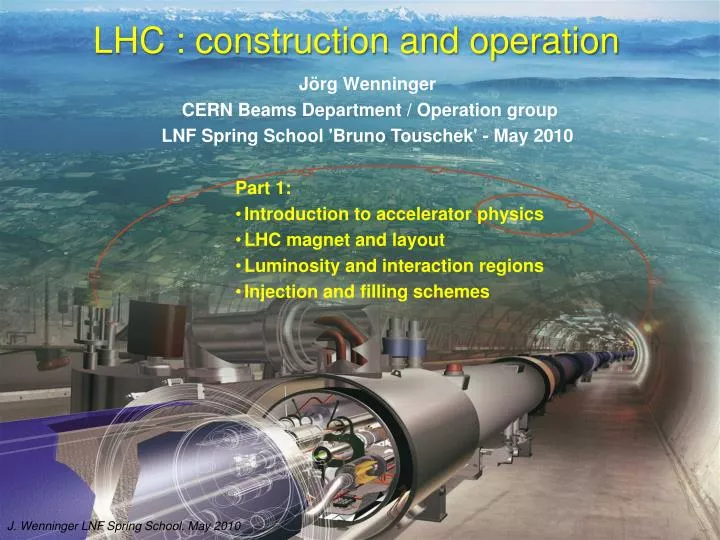
LHC : construction and operation. J örg Wenninger CERN Beams Department / Operation group LNF Spring School 'Bruno Touschek ' - May 2010. Part 1: Introduction to accelerator physics LHC magnet and layout Luminosity and interaction regions Injection and filling schemes. Outline.

E N D
LHC : construction and operation JörgWenninger CERN Beams Department / Operation group LNF Spring School 'Bruno Touschek' - May 2010 • Part 1: • Introduction to accelerator physics • LHC magnet and layout • Luminosity and interaction regions • Injection and filling schemes J. Wenninger LNF Spring School, May 2010
Outline • The LHC challenges • Introduction to magnets and particle focusing • LHC magnets and arc layout • LHC luminosity and interaction regions • Injection and filling schemes • Machine protection • Incident 19th Sept. 2008 and consequences • LHC operation Part 1 Part 2 J. Wenninger LNF Spring School, May 2010
LHC History 1982 : First studies for the LHC project 1983 : Z0/W discovered at SPS proton antiproton collider (SppbarS) 1989 : Start of LEP operation (Z/W boson-factory) 1994 : Approval of the LHC by the CERN Council 1996 : Final decision to start the LHC construction 2000 : Last year of LEP operation above 100 GeV 2002 : LEP equipment removed 2003 : Start of LHC installation 2005 : Start of LHC hardware commissioning 2008 : Start of (short) beam commissioning Powering incident on 19th Sept. 2009 : Repair, re-commissioning and beam commissioning 2010 : Start of a 2 year run at 3.5 TeV/beam J. Wenninger LNF Spring School, May 2010
The Large Hadron Collider LHC Installed in the 26.7 km LEP tunnel Depth of 70-140 m Lake of Geneva LHC ring CMS, Totem LHCb Control Room SPS ring ATLAS, LHCf ALICE Der LHC Beschleuniger - DPG - Bonn
Tunnel circumference 26.7 km, tunnel diameter 3.8 m Depth : ~ 70-140 m – tunnel is inclined by ~ 1.4% J. Wenninger LNF Spring School, May 2010
LHC Layout • 8 arcs. • 8 straight sections (LSS), • ~ 700 m long. • The beams exchange their positions (inside/outside) in 4 points to ensure that both rings have the same circumference ! IR5:CMS Beam1 Beam2 Beam dump blocks IR6: Beam dumping system IR4: RF + Beam instrumentation IR3: Momentum collimation (normal conducting magnets) IR7: Betatron collimation (normal conducting magnets) IR8: LHC-B IR2:ALICE IR1: ATLAS Injection ring 1 Injection ring 2 J. Wenninger LNF Spring School, May 2010
LHC – yet another collider? • The LHC surpasses existing accelerators/colliders in 2 aspects : • The energy of the beam of 7 TeV that is achieved within the size constraints of the existing 26.7 km LEP tunnel. • LHC dipole field 8.3 T • HERA/Tevatron ~4 T • The luminosity of the collider that will reach unprecedented values for a hadron machine: • LHC pp ~ 1034 cm-2 s-1 • Tevatron pp 3x1032 cm-2 s-1 • SppbarS pp 6x1030 cm-2 s-1 • The combination of very high field magnets and very high beam intensities required to reach the luminosity targets makes operation of the LHC a great challenge ! A factor 2 in field A factor 4 in size A factor 30 in luminosity J. Wenninger LNF Spring School, May 2010
Luminosity challenges The event rate N for a physics process with cross-section s is proprotional to the collider Luminosity L: k = number of bunches = 2808 N = no. protons per bunch = 1.15×10¹¹ f = revolution frequency = 11.25 kHz s*x,s*y = beam sizes at collision point (hor./vert.) = 16 mm • To maximize L: • Many bunches (k) • Many protons per bunch (N) • A small beam size s*u = (b*e)1/2 • b*: the beam envelope (optics) • e: is the phase space volume occupied by the beam (constant along the ring). High beam “brillance” N/e (particles per phase space volume) Injector chain performance ! Small envelope Strong focusing ! Optics property Beam property J. Wenninger LNF Spring School, May 2010
Basics of accelerator physics J. Wenninger LNF Spring School, May 2010
Accelerator concept Charged particles are accelerated, guided and confined by electromagnetic fields. - Bending: Dipole magnets - Focusing: Quadrupole magnets - Acceleration: RF cavities In synchrotrons, they are ramped together synchronously to match beam energy. - Chromatic aberration: Sextupole magnets J. Wenninger LNF Spring School, May 2010
→ → → → Force Lorentz force Magnetic rigidity LHC: ρ = 2.8 km given by LEP tunnel! Bending • To reach p = 7 TeV/c given a bending radius of r = 2805 m: • Bending field : B = 8.33 Tesla • Superconducting magnets • To collide two counter-rotating proton beams, the beams must be in separate vaccum chambers (in the bending sections) with opposite B field direction. • There are actually 2 LHCs and the magnets have a 2-magnets-in-one design! J. Wenninger LNF Spring School, May 2010
B field p B I F force I I F p B Bending Fields Two-in-one magnet design J. Wenninger LNF Spring School, May 2010
N S Fy By Fx S N Focusing Transverse focusing is achieved with quadrupolemagnets, which act on the beam like an optical lens. Linear increase of the magnetic field along the axes (no effect on particles on axis). Focusing in one plane, de-focusing in the other! x y J. Wenninger LNF Spring School, May 2010 13
Accelerator lattice horizontal plane Focusing in both planes is achieved by a succession of focusing and de-focusing quadrupole magnets : The FODO structure vertical plane
s y x Alternating gradient lattice One can find an arrangement of quadrupole magnets that provides net focusing in both planes (“strong focusing”). Dipole magnets keep the particles on the circular orbit. Quadrupole magnets focus alternatively in both planes. The lattice effectively constitutes a particle trap! J. Wenninger LNF Spring School, May 2010
LHC arc lattice • Dipole- und Quadrupol magnets • Provide a stable trajectory for particles with nominal momentum. • Sextupole magnets • Correct the trajectories for off momentum particles (‚chromatic‘ errors). • Multipole-corrector magnets • Sextupole - and decapole corrector magnets at end of dipoles • Used to compensate field imperfections if the dipole magnets. To stabilize trajectories for particles at larger amplitudes – beam lifetime ! One rarely talks about the multi-pole magnets, but they are essential for good machine performance ! J. Wenninger LNF Spring School, May 2010
QF QF QF QF QD QD QD Betatron functions in a simple FODO cell Beam envelope • The focusing structure (mostly defined by the quadrupoles: gradient, length, number, distance) defines the transverse beam envelope. • The function that describes the beam envelope is the so-called ‘b’-function (betatron function): • In the LHC arcs the optics follows a regular pattern – regular FODO structure. • In the long straight sections, the betatron function is less regular to fulfill various constraints: injection, collision point focusing… The envelope peaks in the focusing elements ! Horizontal Vertical J. Wenninger LNF Spring School, May 2010
Beam emittance and beam size • For an ensemble of particles: • The transverse emittance, ε, is the area of the phase-space ellipse. • Beam size = projection on X (Y) axis. • The beam size s at any point along the accelerator is given by (neglecting the contribution from energy spread): For unperturbed proton beams, the normalized emittance en is conserved: g = Lorentz factor The beam size shrinks with energy: J. Wenninger LNF Spring School, May 2010
Why does the transverse emittance shrink? • The acceleration is purely longitudinal, i.e the transverse momentum is not affected: • The emittance is nothing but a measure of <pt>. • To maintain the focusing strength, all magnetic fields are kept proportional to E (g), including the quadrupole gradients. • With constant <pt> and increasing quadrupole gradients, the transverse excursion of the particles becomes smaller and smaller ! J. Wenninger LNF Spring School, May 2010
LHC beam sizes • Beta-function at the LHC ARC • Nominal LHC normalized emittance : Example LHC arc, peak b = 180 m J. Wenninger LNF Spring School, May 2010
Acceleration • Acceleration is performed with electric fields fed into Radio-Frequency (RF) cavities. RF cavities are basically resonators tuned to a selected frequency. • To accelerate a proton to 7 TeV, a 7 TV potential must be provided to the beam: • In circular accelerators the acceleration is done in small steps, turn after turn. • At the LHC the acceleration from 450 GeV to 7 TeV lasts ~20 minutes, with an average energy gain of ~0.5 MeV on each turn. s J. Wenninger LNF Spring School, May 2010
LHC RF system • The LHC RF system operates at 400 MHz. • It is composed of 16 superconducting cavities, 8 per beam. • Peak accelerating voltage of 16 MV/beam. • For LEP at 104 GeV : 3600 MV/beam ! The nominal LHC beam radiates a sufficient amount of visible photons to be actually observable ! (total power ~ 0.2 W/m) J. Wenninger LNF Spring School, May 2010
Visible protons ! • Some of the energy radiation by the LHC protons is emitted as visible light. It can be extracted with a set of mirrors to image the beams in real time. • This is a powerful tool to understand the beam size evolution. Protons are very sensitive to perturbations, keeping their emittance small is always a challenge. Flying wire LHC Synch. light Flying wire SPS (injector) J. Wenninger LNF Spring School, May 2010
Cavities in the tunnel J. Wenninger LNF Spring School, May 2010
RF buckets and bunches The particles oscillate back and forth in time/energy The particles are trapped in the RF voltage: this gives the bunch structure RF Voltage 2.5 ns time E LHC bunch spacing = 25 ns = 10 buckets 7.5 m RF bucket time 2.5 ns 450 GeV 3.5 TeV RMS bunch length 12.8 cm 5.8 cm RMS energy spread 0.031% 0.02% J. Wenninger LNF Spring School, May 2010
Magnets & Tunnel J. Wenninger LNF Spring School, May 2010
Superconductivity • The very high DIPOLE field of 8.3 Tesla required to achieve 7 TeV/c can only be obtained with superconducting magnets ! • The material determines: Tccritical temperature Bc critical field • The cable production determines: • Jc critical current density • Lower temperature increased current density higher fields. • Typical for NbTi @ 4.2 K 2000 A/mm2 @ 6T • To reach 8-10 T, the temperature must be lowered to 1.9 K – superfluid Helium ! Bc Tc J. Wenninger LNF Spring School, May 2010
The superconducting cable 6 m 1 mm A.Verweij Typical value for operation at 8T and 1.9 K: 800 A width 15 mm Rutherford cable A.Verweij J. Wenninger LNF Spring School, May 2010
Coils for dipoles Dipole length 15 m I = 11’800 A @ 8.3 T The coils must be aligned very precisely to ensure a good field quality (i.e. ‘pure’ dipole) J. Wenninger LNF Spring School, May 2010
Ferromagnetic iron Non-magnetic collars Superconducting coil Beam tube Steel cylinder for Helium Insulation vacuum Vacuum tank Supports Weight (magnet + cryostat) ~ 30 tons, length 15 m J. Wenninger LNF Spring School, May 2010 Rüdiger Schmidt 30
Regular arc: Magnets 1232 main dipoles + 3700 multipole corrector magnets (sextupole, octupole, decapole) 392 main quadrupoles + 2500 corrector magnets (dipole, sextupole, octupole) J. Wenninger LNF Spring School, May 2010 J. Wenninger - ETHZ - December 2005 31
Connection via service module and jumper Static bath of superfluid helium at 1.9 K in cooling loops of 110 m length Supply and recovery of helium with 26 km long cryogenic distribution line Regular arc: Cryogenics J. Wenninger LNF Spring School, May 2010 J. Wenninger - ETHZ - December 2005 32
Beam vacuum for Beam 1 + Beam 2 Insulation vacuum for the magnet cryostats Insulation vacuum for the cryogenic distribution line Regular arc: Vacuum J. Wenninger LNF Spring School, May 2010 J. Wenninger - ETHZ - December 2005 33
Tunnel view (1) J. Wenninger LNF Spring School, May 2010
Tunnel view (2) J. Wenninger LNF Spring School, May 2010
Complex interconnects Many complex connections of super-conducting cable that will be buried in a cryostat once the work is finished. This SC cable carries 12’000 A for the main quadrupole magnets J. Wenninger LNF Spring School, May 2010 CERN visit McEwen
Magnet cooling scheme • He II: super-fluid • Very low viscosity • Very high thermal conductivity Courtesy S. Claudet J. Wenninger LNF Spring School, May 2010
Cryogenics 8 x 18kW @ 4.5 K 1’800 SC magnets 24 km & 20 kW @ 1.8 K 36’000 t @ 1.9K 130 t He inventory Courtesy S. Claudet Grid power ~32 MW J. Wenninger LNF Spring School, May 2010
Cool down Cool-down time to 1.9 K is nowadays ~4 weeks/sector [sector = 1/8 LHC] J. Wenninger LNF Spring School, May 2010
Vacuum chamber • The beams circulate in two ultra-high vacuum chambers, P ~ 10-10 mbar. • A Copper beam screen protects the bore of the magnet from heat deposition due to image currents, synchrotron light etc from the beam. • The beam screen is cooled to T = 4-20 K. 50 mm 36 mm Beam screen Magnet bore Cooling channel (Helium) Beam envel ( 4 s) ~ 1.8 mm @ 7 TeV J. Wenninger LNF Spring School, May 2010
Luminosity and interaction regions J. Wenninger LNF Spring School, May 2010
Luminosity • Let us look at the different factors in this formula, and what we can do to maximize L, and what limitations we may encounter !! • f : the revolution frequency is given by the circumference, f=11.246 kHz. • N : the bunch population – N=1.15x10¹¹ protons • - Injectors (brighter beams) • - Collective interactions of the particles • - Beam encounters • k : the number of bunches – k=2808 • - Injectors (more beam) • - Collective interactions of the particles • - Interaction regions • - Beam encounters • s* : the size at the collision point –s*y=s*x=16 mm • - Injectors (brighter beams) • - More focusing – stronger quadrupoles For k = 1: J. Wenninger LNF Spring School, May 2010
Collective (in-)stability • The electromagnetic fields of a bunch interact with the vacuum chamber walls (finite resistivity !), cavities, discontinuities etc that it encounters: • The fields act back on the bunch itself or on following bunches. • Since the fields induced by of a bunch increase with bunch intensity, the bunches may become COLLECTIVELY unstable beyond a certain intensity, leading to poor lifetime or massive looses intensity loss. • Such effects can be very strong in the LHC injectors, and they will also affect the LHC – in particular because we have a lot of carbon collimators (see later) that have a very bad influence on beam stability ! • limits the intensity per bunch and per beam ! J. Wenninger LNF Spring School, May 2010
‘Beam-beam’ interaction • When a particle of one beam encounters the opposing beam at the collision point, it senses the fields of the opposing beam. • Due to the typically Gaussian shape of the beams in the transverse direction, the field (force) on this particle is non-linear, in particular at large amplitudes. • focal length depends on amplitude ! • The effect of the non-linear fields can become so strong (when the beams are intense) that large amplitude particles become unstable and are lost from the machine: • poor lifetime • background • THE INTERACTION OF THE BEAMS SETS A LIMIT ON THE BUNCH INTENSITY! Quadrupole lens Beam(-beam) lens J. Wenninger LNF Spring School, May 2010
From arc to collision point CMS collision point ARC cells ARC cells Fits through the hole of a needle! • Collision point size @ 7 TeV, b* = 0.5 m (= b-function at the collision point): • CMS & ATLAS : 16 mm • Collision point size @ 3.5 TeV, b* = 2 m: • All points : 45 mm J. Wenninger LNF Spring School, May 2010
Limits to b* Small size • The more one squeezes the beam at the IP (smaller b*) the larger it becomes in the surrounding quadrupoles (‘triplets’): Huge size !! Huge size !! • Smaller the size at IP: • Larger divergence (phase space conservation !) • Faster beam size growth in the space from IP to first quadrupole ! • Aperture in the ‘triplet’ quadrupoles around the IR limits the focusing ! J. Wenninger LNF Spring School, May 2010
Combining the beams for collisions • The 2 LHC beams must be brought together to collide. • Over ~260 m, the beams circulate in the same vacuum chamber. They are ~120 long distance beam encounters in total in the 4 IRs. J. Wenninger LNF Spring School, May 2010
IP Crossing angles • Since every collision adds to our ‘Beam-beam budget’ we must avoid un-necessary direct beam encounters where the beams share a common vacuum: • COLLIDE WITH A CROSSING ANGLE IN ONE PLANE ! • There is a price to pay - a reduction of the luminosity due to the finite bunch length and the non-head on collisions: • L reduction of ~17% • Crossing planes & angles • ATLAS Vertical 280 mrad • CMS Horizontal 280 mrad • LHCb Horizontal 300 mrad • ALICE Vertical 400 mrad 7.5 m J. Wenninger LNF Spring School, May 2010
Separation and crossing : example of ATLAS Horizontal plane: the beams are combined and then separated ATLAS IP 194 mm ~ 260 m Common vacuum chamber Vertical plane: the beams are deflected to produce a crossing angle at the IP Not to scale ! ~ 7 mm J. Wenninger LNF Spring School, May 2010
Tevatron J. Wenninger LNF Spring School, May 2010