Download
1 / 32
320 likes | 459 Views
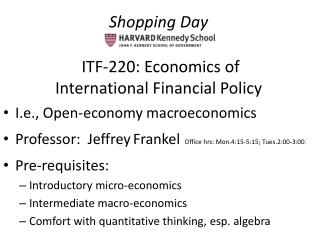
Economics of International Financial Policy: ITF 220. Staff -- Professor: Jeffrey Frankel , Littauer 217 Office hours: Mondays 4:15-5:15; Tuesdays 2:00-3:00. Faculty Asst.: Minoo Ghoreishi, Belfer 505 (617) 384-7329 Teaching Fellow: Tilahun Emiru

E N D
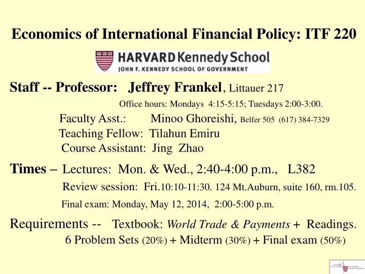
Economics of International Financial Policy: ITF 220 Staff -- Professor: Jeffrey Frankel,Littauer 217 Office hours: Mondays 4:15-5:15; Tuesdays 2:00-3:00.Faculty Asst.: Minoo Ghoreishi, Belfer 505 (617) 384-7329 Teaching Fellow: Tilahun Emiru Course Assistant: Jing Zhao Times – Lectures: Mon. & Wed., 2:40-4:00 p.m., L382 Review session: Fri.10:10-11:30.124 Mt.Auburn, suite 160, rm.105. Final exam: Monday, May 12, 2014, 2:00-5:00 p.m. Requirements -- Textbook: World Trade & Payments + Readings. 6 Problem Sets (20%) + Midterm (30%) + Final exam (50%) .
Big topics covered in the course I) ELASTICITIES & THE TRADE BALANCE II) THE KEYNESIAN MODEL OF INCOME • THE MONETARY APPROACH TO THE BALANCE OF PAYMENTS IV) GLOBALIZATION OF FINANCIAL MARKETS V) FISCAL & MONETARY POLICY UNDER INTERNATIONAL CAPITAL MOBILITY VI) INTERDEPENDENCE AND COORDINATION VII) SUPPLY, INFLATION & MONETARY UNION VIII) EXPECTATIONS, MONEY, & DETERMINATION OF THE EXCHANGE RATE Professor Jeffrey Frankel, Kennedy School, Harvard University
TOPIC I: ELASTICITIES & THE TRADE BALANCE • Lecture 1: Balance of Payments Accounting • Lecture 2: Supply & demand for foreign exchange; export and import elasticities • Lecture 3: Empirical effects of devaluation on the trade balance
Lecture 1:Balance of payments accounting • Definition: The balance of payments is the year’s record of economic transactions between domestic and foreign residents. • The rules: • If you have to pay a foreign resident, normally in exchange for something that you bring into the country, then the something counts as a debit. • If a foreign resident has to pay you for something, then the something counts as a credit. Professor Jeffrey Frankel, Kennedy School, Harvard University
† † Now also called “financial account” Professor Jeffrey Frankel, Kennedy School, Harvard University
PER QUARTER Measures of external balanceUS 2004-2013 Current Account Goods &Services Goods US services surplus partially offsets the deficit in goods. Professor Jeffrey Frankel, Kennedy School, Harvard University
Examples on the current account: • You, an American, import software CD-roms from India=> debits appear on US merchandise account. • You import services (electronically) of an Indian software firm=> debit appears on US services account.(This is the famous and controversial “overseas outsourcing.”) • You buy the services, instead, from a subsidiary that the Indian software firm set up last year in the US. This is not an international transaction, and so does not appear in the accounts. But assume the subsidiary sends some profits back to India => debit appears on US investment income account.(It is as if the US is paying for the services of Indian capital.) • Employees of the subsidiary in the US (or any other US resident entities) send money to relatives back in India => debit appears under unilateral transfers. Professor Jeffrey Frankel, Kennedy School, Harvard University
Examples on the long-term capital account: • Instead of buying software CD-roms from India, you buy the company in India that makes them. => debit appears on US capital account, under FDI. (You have imported ownership of the company.) • Instead of buying the entire company in India, you buy some stock in it => debit appears on US capital account, under equities.(You have imported claims against an Indian resident.) • Instead of buying stock in the company, you lend it money for 2 years => debit appears on US capital account, under bonds or bank loans.(Again, you have imported a claim against an Indian resident.) Professor Jeffrey Frankel, Kennedy School, Harvard University
Examples on the short-term capital account: • You lend to the Indian company in the form of 30-day commercial paper or trade credit => debit appears on US short-term capital account.(Again, you have acquired a claim against India.) • You lend to the Indian company in the form of cash dollars, which they don’t have to pay back for 30 days => debit appears on US short-term capital account. • You are the Central Bank, and you buy securities of the Indian company (an improbable example for the Fed – but “Sovereign Wealth Funds,” from China to oil-exporting countries, now make international investments of this sort)=> debit appears as a US official reserves transaction. Professor Jeffrey Frankel, Kennedy School, Harvard University
The rules, continued Each transaction is recorded twice: once as a credit and once as a debit. E.g., when an importer pays cash dollars, the debit on the merchandise account is offset by a credit under short-term capital: the exporter in the other country has, at least for the moment, increased holdings of US assets, which counts as a credit just like any other portfolio investment in US assets. At the end of each quarter, credits & debits are added up within each line-item; and line-items are cumulated from the top to compute measures of external balance. Professor Jeffrey Frankel, Kennedy School, Harvard University
Some balance of payments identities CA ≡ Rate of increase in net international investment position. CA-surplus country (Japan) accumulates claims against foreigners; CA-deficit country (US) borrows from foreigners. CA + KA + ORT ≡ 0 . BoP ≡ CA + KA . => BoP ≡ -ORT ≡ excess supply of FX coming from private sector, (i.e., all credits from exports of goods,services, assets… minus all debits)which central banks absorb into reserves, if they intervene in FX market). A BoPsurplus country (China, Saudi A.) adds to its FX reserves A BoP deficit country (Argentina) either runs down its FX reserves or, is lucky enough for foreign central banks to finance the deficit, if its currency is an international reserve asset (US $) . A floating country (Japan, Chile) does not intervene in the FX market => BP ≡ 0; Exchange rate E adjusts to clear FX supply & demand in private market
End of Lecture 1: Balance of Payments Accounting Professor Jeffrey Frankel, Kennedy School, Harvard University
Lecture 2: The Elasticities Approach to the Trade Balance • Primary question: Under what circumstances does devaluation improve the trade balance (TB), and how much? • Secondary question: If the currency floats(i.e., the central bank does not intervene in the foreign exchange market),how much must the exchange rate (E) move to clear the trade balance by itself? • Model: Elasticities Approach • Keyequation: Marshall-Lerner Condition Professor Jeffrey Frankel, Kennedy School, Harvard University
Supply & demand for foreign exchange DS E ≡price offoreignexchange in $/₤ FX supply arises from exports, capital inflows… FX demand arises from imports, capital outflows… Quantity of foreign exchange, ₤ Professor Jeffrey Frankel, Kennedy School, Harvard University
Assume demand for forex shifts out e.g., to due to increase in demand to buy foreign goods or assets Deficit (excess demand for foreign currency) Depreciation(increase in price of foreign currency) Professor Jeffrey Frankel, Kennedy School, Harvard University
The Elasticities Approach to the Trade Balance • derives the supply of foreign exchange from export earnings, and • derives the demand for foreign exchange from import spending. • Capital flows are not considered (until later), so no supply of, or demand for, FX comes from international borrowing or lending. Professor Jeffrey Frankel, Kennedy School, Harvard University
How the Exchange Rate, E, Influences BoP • Supply of FX determined by EXPORT earnings • Demand for FX determined by IMPORT spending • No capital flowsor transfers=> BoP = TB 2) PCP: Price in termsof producer’s currency;Supply elasticity = ∞ . => Domestic firms set . & Foreign firms set . 3) Complete exchange rate passthrough: Price of X in foreign currency = / E Price of Imports in domestic currency = E 4) Demandis adecreasing function of price in consumer’s currency => IM= IMD (E ) . => X = XD ( / E ) . => Net supply of FX = TB expressed in foreigncurrency ≡ TB* = ( /E) XD( /E) - ( ) IMD(E ) . Professor Jeffrey Frankel, Kennedy School, Harvard University
How the TB is affected by the exchange rate (continued) TRADE BALANCE EXPRESSED IN FOREIGN CURRENCY TB* = ( /E) XD( /E) - ( ) IMD(E ) . EXPERIMENT : E↑ • THREE EFFECTS (1) IMD( ) falls. EFFECT ON TB* + + - (2) XD( ) rises. (3) Price of X in terms of foreign currency falls. NET EFFECT ON TB* is determined by Marshall-Lerner condition. Add one more assumption: Before the devaluation, TB*=0, so export earnings cancel out import spending, Then devaluation improves the TB iff: εX+εM> 1 .
Example (i) to illustrate Marshall-Lerner condition for TB* = ( /E) XD( /E) - ( ) IMD(E ) • If εx =1, then E↑ leaves export revenue unchanged. • Because effects (2) and (3) cancel out. • In that case, so long as εM > 0, • Marshall-Lerner condition is satisfied: • Import spending falls -- effect (1) -- • TB* improves. Professor Jeffrey Frankel, Kennedy School, Harvard University
Example (ii) to illustrate Marshall-Lerner condition for TB* = ( /E) XD( /E) - ( ) IMD(E ) . • If εx = 0, then E ↑ cuts export revenue in proportion • because of valuation effect (3) • In that case, is εM > 1 necessary to improve TB* ? • Yes, because of Marshall-Lerner condition • -- fall in import spending then outweighs fall in export revenue: effect (1) > effect (2) -- • provided initial X revenue > import spending. • But if initial TB*<0, elasticities need not be as high. Professor Jeffrey Frankel, Kennedy School, Harvard University
How the TB is affected by the exchange rate (continued) TRADE BALANCE EXPRESSED IN DOMESTIC CURRENCY TB = ( ) XD( /E) -(E ) IMD(E ) . EXPERIMENT : E↑ • THREE EFFECTS (2) IMD( ) falls. EFFECT ON TB + + - (1) XD( ) rises. (3) Price of IMports in terms of domestic currency rises. NET EFFECT ON TBis determined by the same Marshall-Lerner condition. Again, assume that initially TB=0. Then devaluation improves the TB iff: εX+εM> 1 .
End of Lecture 2: Elasticities Approach to the Trade Balance Professor Jeffrey Frankel, Kennedy School, Harvard University
Lecture 3: Empirical effects of devaluation on the trade balance • Examples:Italy after 1992; Poland after 2008. • Elasticity Pessimism: • Countries often fear their elasticities are too low for the M-L condition. • Econometric estimation of elasticities• What is OLS regression?• Typical estimates• The importance of lags. • The J-curve•With fast pass-through to import prices • With slow pass-through to import prices . Professor Jeffrey Frankel, Kennedy School, Harvard University
1992 devaluation Rise in trade balance Professor Jeffrey Frankel, Kennedy School, Harvard University
Depreciation boosted net exports => Poland avoided recession, alone in EU Poland’s exchange rate rose 35% in the 2008-09 global crisis. Exchange rate Zloty / € Contribution of Net X in 2009: 3.1 % of GDP >Total GDPgrowth:1.7% Source: Cezary Wójcik
. . . . . . . . . . X ≡ Exports demanded How can we estimate sensitivity of export demand to exchange rate?OLS regression EP*/P ≡ Price of foreign goods relative to domestic goods Professor Jeffrey Frankel, Kennedy School, Harvard University
Common econometric finding Estimated trade elasticities with respect to relative prices often ≈ 1, after a few years have been allowed to pass. => Marshall-Lerner condition holds in the medium run. Some face a higher elasticity of demand for their exports: small countries, and producers of agricultural & mineral commodities or other commodities that are close substitutes for competitors’ exports.
Common empirical observation: After a devaluation, trade balance gets worse before it gets better. Explanation: Even if devaluation is instantly passed throughto higher import prices, buyers react with a lag. Also, in practice, it often takes time before the devaluation is passed through to import prices.
End of Lecture 3: Empirical Effects of Devaluation on the Trade Balance Professor Jeffrey Frankel, Kennedy School, Harvard University
Appendix:Determinants of US TB • 1980 deficits: Effects of • $ appreciation of 1980-85 (“Reaganomics”) • $ depreciation of 1985-87 (Plaza Accord). • Subsequent deficits:Effects of • $ appreciation of 1995-97 Professor Jeffrey Frankel, Kennedy School, Harvard University
US TB & CA, 2001-2010, $ millions • The deficits shranksharply in 2008-09, • due to: • lagged effects of $depreciation 2002-07 • and the recession. Professor Jeffrey Frankel, Kennedy School, Harvard University
US trade and current account balances 1970-2010 ($ millions) ↑ Surplus ↓ Deficit Services always partiallyoffset the deficit in goods. The US trade balance was on a downward trend, 1965-2011 despite a few temporary improvements (including during recessions: 1990-91, 2001, & especially 2008-09) Professor Jeffrey Frankel, Harvard University