Download
1 / 27
270 likes | 375 Views
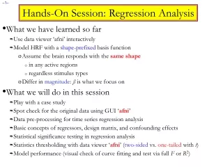
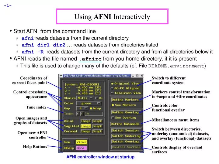
Using AFNI Interactively. Start AFNI from the command line afni reads datasets from the current directory afni dir1 dir2 … reads datasets from directories listed afni -R reads datasets from the current directory and from all directories below it

E N D
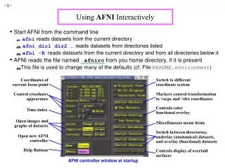
Using AFNI Interactively • Start AFNI from the command line • afni reads datasets from the current directory • afni dir1 dir2 … reads datasets from directories listed • afni -R reads datasets from the current directory and from all directories below it • AFNI reads the file named .afnirc from you home directory, if it is present • This file is used to change many of the defaults (cf. File README.environment) Coordinates of current focus point Switch to different coordinate system Control crosshairs appearance Markers control transformation to +acpc and +tlrc coordinates Controls color functional overlay Time index Open images and graphs of datasets Miscellaneous menu items Switch between directories, underlay (anatomical) datasets, and overlay (functional) datasets Open new AFNI controller Help Buttons Controls display of overlaid surfaces AFNI controller window at startup
Miscellaneous features of the AFNI controller window: • xyz-coordinate display in upper left corner shows current focus location • By default, the coordinates are in RAI order (from the DICOM standard): • x = Right (negative) to Left (positive) • y = Anterior (negative) to Posterior (positive) • z = Inferior (negative) to Superior (positive) • This display order can be changed to the neuroscience imaging order LPI: • x = Left (negative) to Right (positive) • y = Posterior (negative) to Anterior (positive) • z = Inferior (negative) to Superior (positive) • The [Bhelp] button: when pressed, the cursor changes to a hand shape; use it to click on any AFNI button and you will get a small help popup • AFNI also has ‘hints’ (AKA ‘tooltips’) • Press the [New] button to open a new AFNI controller • Used to look at more than one dataset at a time • [Define Datamode][Lock] can be used to lock controllers together by coordinates • All viewing windows within a controller are always locked together • Press the [Views] button to close/open the control panel at right
Press the [done] button twice within 5 seconds to exit AFNI • The first button press changes ‘done’ to ‘DONE’ • Fail to press second time in 5 seconds and it changes back to ‘done’ • Whatever you do, don’t press a mouse button in the blank area to the right of [done] • I won’t be responsible for the consequences • The [Switch] buttons let you control which datasets are being viewed • [Switch Session] controls which directory datasets are drawn from • [Switch Underlay] control the background (grayscale) dataset --- anat dataset usually goes here • Current anat dataset determines the resolution of and 3D region covered by image viewers • [Switch Overlay] controls the overlay (color) dataset --- func dataset usually goes here • Func datasets will be interpolated -- if needed -- to anat resolution, and flipped -- if needed -- to anat orientation • Current datasets are named in AFNI controller titlebar
Touring the Image Viewer Image viewer; Disp and Mont control panels
Crosshairs show the current focus location • Also show the cut planes for the other image viewers • When using image montage, other viewers show multiple crosshairs • Can control crosshair color and gap size from main AFNI controller • Slider below image lets you move between slices • Left-click and drag ‘thumb’ to move past many slices • Left-click ahead or behind thumb to move 1 image at a time • Hold click down to scroll continuously through slices • Middle-click in ‘trough’ to jump quickly to a given location • Vertical intensity bar to right of image shows mapping from numbers stored in image to colors shown on screen • Bottom of intensity bar corresponds to smallest numbers displayed • Top corresponds to largest numbers displayed • Smallest-to-largest display range is selected from [Disp]control panel • or from hidden popup menu on intensity bar • All image viewers from all AFNI controllers use the same intensity bar • unless AFNI is started with the -uniq command line option, in which case each AFNI controller’s viewers have independent intensity bars • but all image viewers from the same controller always share the same intensity bar
Buttons at right • [Colr] changes grayscale to color spectrum, and back • [Swap] swaps top of intensity bar with bottom • [Norm] returns the intensity bar to normal (after you mess it up) • [c] controls contrast • [b] controls brightness • Useful combination [c]5 2-3 times, [b]6 2-3 times • [R] rotates the intensity bar (useless, but very fun) • [g] changes the gamma factor (nonlinearity) for the intensity bar • [I] changes the size of the image in the window • [9] changes the opacity of the color overlay • This control only present for X11 TrueColor displays • At bottom right, the arrowpad controls the crosshairs • Arrows move 1 pixel in that direction for that window • Sagittal 3 is same as Axial 5 • Central button closes and opens crosshair gap • Items on AFNI controller (below xzy display) also alter crosshairs • Can change color, gap size, …
Buttons along bottom provide various services • [Disp] controls the way images are displayed and saved • Pops up its own control window: most controls change image immediately • Orientation controls at top allow you to flip image around • [No Overlay] lets you turn color overlays off (crosshairs; function) • [Min-to-Max] intensity bar is data min-to-max • [2%-to-98%] intensity bar is smallest 2% of data to largest 98% • [Free Aspect] lets you distort image shape freely • [Save panel] controls how images are saved to disk: • All buttons off saved image file contains slice raw data • [Nsize Save] same, but images are 2N in size • [PNM Save] images are saved in PPM/PGM format (color/gray) • [Save to .xxx(s)] saves image(s) to specified format • [Save One] for saving montage • [Tran 0D] lets you transform voxel values before display • [Log10] and [SSqrt] useful for images with extreme values • [Tran 2D] provides some 2D image filters (underlay only) • [Median 9] smoothing can be useful for printing images • [Rowgraphs]lets you graph the voxel values from image rows • If you want columns, flip the image with [CCW 90] • [Surfgraph] lets you graph the voxel values in a surface graph
Three extra imaging processing filters are provided at the bottom • [Sharpen] is sometimes useful for deblurring images • [Reset] sets controls back to what they were when you opened [Disp] • [Done] closes this control window • [Save] lets you save images from viewer to disk files • Warning: Images are saved as sent to the viewer, not as displayed • Means that aspect ratio of saved image may be wrong (non-square pixels) • Can fix this with [Define Datamode][Warp Anat on Demand] • [Save:bkg] means it will save the background image data itself, whatever the format it may be in (bytes, shorts, floats, complex numbers, RGB byte triples) • [Save:pnm] means it will save the displayed image in PNM format • PPM for color, PGM for gray-only images • You might have to convert this to some other format • See AFNI FAQ #57 for instructions on image format conversion • [Sav1:xxx] means it will save the entire Montage in format “xxx” • This is the only way to save a Montage layout (within AFNI) • [Save] options will only save single slice images (one or more) • [Save.xxx] means it will save the image in the “xxx” format • You can also set this using the hidden right-click popup on the [Save] Button • Formats depend on presence of image conversion programs on your system
After you press [Save], then it asks for a filename prefix • Except for [Sav1.xxx], it then asks for ‘from’ and ‘to’ slice indexes • You can save many images this way • Filenames are like are like prefix.0037.ppm, for slice #37, ppm format • [Sav1.xxx] immediately saves its one file after prefix is entered • [Mont] lets you display a rectangular layout of images (i.e., montage) • Pops up its own little control window • Controls at top do nothing until an action is selected at bottom • [Across] and [Down] determine number of sub-images shown • [Spacing] determines how far apart the selected slices are • Every nth slice, for n = 1, 2, … • Multiple crosshairs in other image viewers will show montage slices • [Border] lets you put some blank pixels between sub-images • [Color] lets you choose the color of the border pixels • At the bottom, the action controls cause something to happen: • [Quit] closes the Montage control window • [1x1] changes Across and Down back to 1 • [Draw] actually causes the montage to be drawn • [Set][Draw] then [Quit]
[Rec] lets you record images for later Save-ing • So you can build a sequence of images from any set of AFNI controls • Change color maps, functional thresholds, datasets, … • Then save them to disk for animation, etc. • If Unix programs whirlgif and/or gifsicle are installed on your system, AFNI can write GIF animations directly (e.g., for fun Web pages) • If program mpeg_encode is installed, AFNI can write MPEG-1 animations • Source code for these free programs is included with AFNI source code • [Rec] button pops down a menu that sets the record mode • [Off] recording is off • [Next One] next image displayed is recorded, then goes back to [Off] • [Stay On] record each image when displayed • Controls below the line determine where in the recording sequence the saved images will be stored • Recorded images go into a new image viewer, with its own controls • Its slider moves between recorded images • [Kill] will delete an image from the recorded sequence • [Save] will save record images • Right-click on [Save] to bring up menu of format options • [Done] to close the recorded image viewer
Hidden image popup menu (using Button 3 or right-click) • [Jumpback] lets you jump the focus position back to its last place • For when you click in the wrong place and get lost • [Jump to (xyz)] lets you enter xyz-coordinates (in mm), and then the focus position will jump there • External program 3dclust can generate xyz coordinates of interest • Once you have +tlrc dataset, can jump to regions from Talairach atlas • [Jump to (ijk)] lets you jump to a particular voxel index location • [Image display] lets you turn control widgets on and off • Can unclutter screen a little • Useful if you want to make a screenshot • Hidden intensity bar popup menu • [Choose Display Range] lets you pick the range of numbers that are mapped to intensity bar colors • Normally, each image is mapped to colors separately when it is displayed • Using Min-to-Max or 2%-to-98% from [Disp] • If you want each image to be mapped the same, then must give bottom-to-top values via this menu item (separate them with spaces) • If you set third (optional) input ‘ztop’ to 1, values above ‘top’ are set to 0 • To restore normal auto-mapping, set ‘bot’ and ‘top’ both to 0
[Choose Zero Color] lets you choose the color that is displayed for voxel values that are exactly 0 • Can be useful for filling in regions that were set to 0 by some program • For example, values below ‘bot’ from Choose Display Range (and above ‘top’ if ‘ztop’ was set to 1) • Choose the ‘none’ color to return to normal display • [Choose Flatten Range] is used to control the Flatten filter from the [Disp] control window • This is almost useless --- don’t bother to try it • [Choose Sharpen Factor] is used to control the Sharpen filter from the [Disp] control window • Larger values mean more sharpening (and more image graininess) • [Plot Overlay Plots] turns overlay graphs on and off • In future, will control overlay of cortical surface geometry • This feature is experimental now, and not documented • [Label] and [Size] controls display of slice coordinate overlay
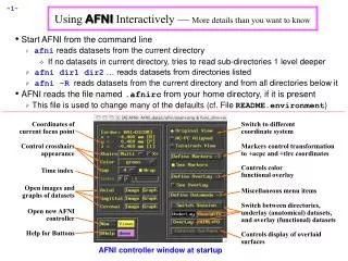
Touring the Graph Viewer Graph Viewer with data (black) and reference waveforms (red)
Graph viewer takes voxel values from same dataset as image viewer • If dataset has only 1 sub-brick, graph viewer only shows numbers • To look at images from one dataset locked to graphs from another dataset, must use 2 AFNI controllers and [Define Datamode] [Lock] on AFNI control panel • If graph and image viewer in same slice orientation are both open, crosshairs in image window change to show a box containing dataset voxels being graphed • Central sub-graph (current focus location) is outlined in yellow • Current time index is marked with small red diamond • Left-clicking in a non-central sub-graph moves that location to focus • Left-clicking in central sub-graph moves time index to that point • Can also use [Index] control in AFNI controller • Right-clicking in any sub-graph pops up some statistics of its data • Left-clicking in icon (lower left corner) causes icon and menu buttons to disappear • Useful if you want to do a screenshot to save window • Left-clicking in same place will bring icon and buttons back
[Opt] menu buttons let you control how graphs appear • Many items have keyboard shortcuts • Make sure you are typing in the correct window! • [Scale] changes scale of graphs • Mapping from voxel values to screen pixels • Down[-] shrinks graphs vertically; Up[+] expands them • Auto[a] makes AFNI pick a nice scale factor • [Choose] lets you pick exact scale factor • Can choose positive values = pix/datum or negative = datum/pix • pix/datum = number of screen pixels for each change of 1 in data • datum/pix = size of change in data for each screen pixel • Current scale factor is shown below graphs • Scale factor does not change when you resize graph,change matrix, etc. • You usually have to auto-scale [a] afterwards • [Matrix] changes number of sub-graphs • Down[m] and Up[M] decrease and increase number • [Choose] lets you pick number exactly • Alternative: keyboard [N], type number, then [Enter] key • Range of allowable matrix size is 1..21
[Grid] lets you change spacing of vertical grid lines • Useful for showing regular timing interval (e.g., task timing) • Down[g] and Up[G] decrease and increase spacing • [Choose] lets you pick number exactly • Current grid spacing is shown below graphs • [Pin Num] lets you pick the horizontal length of the sub-graph • Default length is number of sub-bricks in dataset • Make it longer graphs end before window • Make it shorter graphs are truncated • Useful when switching between datasets of different lengths • Set this to 0 to get back to default operation • Current number of time points is shown below graphs • HorZ[h] will put in a dashed line at the y = 0 level in sub-graphs • Only useful if data range spans negative and positive values! • [Slice] lets you change slices • Down[z] and Up[Z] move one slice • Can also choose slice directly from menu • Current voxel indexes are shown below graphs • Corresponds to [Voxel Coords?] Display in AFNI controller
[Colors, Etc.] lets you alter the colors/lines used for drawing • Lines used for sub-graph frame boxes, grid lines, data graphs, FIM orts/ideals, and double plots can have color changes and be made thicker • Grid color is also used to highlight central sub-graph • Can choose to graph curves as lines, points, or both together • Can change color of background and text • Can change gap between sub-graph boxes • Baseline[b] changes how the sub-graphs are plotted • All sub-graphs have same scale factor, to convert values into vertical pixels • Baseline is value that gets plotted to bottom of sub-graph • Individual: all sub-graphs have different baselines • Baseline = smallest value in each displayed time series • This can be confusing; same vertical location doesn’t mean same value • Shown below graphs as Base: separate • Common: all sub-graphs shown at any one time get same baseline • Baseline = smallest value in all displayed time series • Shown below graphs as Base: common • Usually need to rescale [a] after changing baseline • Global: all sub-graphs get same baseline even when spatial position changes • Set from [Baseline][Set Global] menu item • Default global level is smallest value in entire dataset
Range of central sub-graph is shown at left of graph region • Central bottom (baseline) value is shown at lower left • Upper left shows value at top of central sub-graph box • Number in [brackets] shows data range of one sub-graph box’s height • If baselines are separate, bot/top values only apply to central sub-graph • Show text?[t] allows you to see text display of values instead of graphs • Save PNM[S] lets you save a snapshot of window to a PNM image file • Write Center [w] lets you write data from central sub-graph to a file • File is in ASCII format can be imported into other programs • Filename is of form xxx_yyy_zzz.suffix.1D (using voxel indexes) • Suffix is chosen using [Set ‘w’ suffix] button • [Tran 0D] and [Tran 1D] let you transform the data before graphing • [Log10] and [SSqrt] useful for images with extreme values • [Median3] and [OSfilt3] are for are for smoothing time series • Other choices are functions controlled by/from plugins • [Double Plot] lets you plot output of [Tran 1D] and original data together • Color of transformed data from [Dplot] on the [Colors, Etc.] menu • [Dataset#2] transformation lets you plot two datasets together
[X-axis] menu lets you choose how graph x-axis is chosen • Default: x is linear in time • Can instead choose x from a .1D format file from disk • Useful only in very limited circumstances • Done[q] closes the graph viewer window • Keystrokes in graphs that have no menu items are: • [<] moves time index down by 1 • [>] moves time index up by 1 • [1] moves time index to beginning (time index = 0) • [l] moves time index to end • [L] turns off/on the AFNI logo in the corner • [FIM] menu controls interactive functional image calculations • Not documented here; see ‘Educational materials’ pages at AFNI Web site
Choose which sub-brick from Underlay dataset to display (usu. Anat - has only 1 sub-brick) Color map Hidden popup menu here Choose which dataset makes the underlay image • Brief Tour of the Functional Color Overlay Controls • Open with [Define Overlay] button on AFNI controller Threshold slider Choose which sub-brick of functional dataset makes the color Choose which sub-brick of functional dataset is the Threshold p-value of current threshold Shows ranges of data in Underlay and Overlay dataset Choose range of threshold slider, in powers of 10 Shows automatic range for color scaling Rotates color map Positive-only or both signs of function? Number of panes in color map Shows voxel values at focus Lets you choose range for color scaling
AFNI Plugins • Plugins are modules that attach themselves to AFNI and add some interactive capabilities to the GUI program • There is a (somewhat dated) manual for writing plugins • Useful plugins: • 3D Registration: Provides a GUI control for time series registration (same as 3dvolreg) • Dataset Copy: Copy a dataset (useful as a start for ROI drawing) • Dataset NOTES: Add arbitrary text notes to a dataset header • Draw Dataset, Gyrus Finder: Draw regions-of-interest (ROIs) on 2D slices • Histogram: Graph the histogram of a sub-brick, or some parts of it • Deconvolution, Nlfit & Nlerr: Do linear and nonlinear regression interactively on the dataset time series being displayed in a graph viewer
Pick new underlay dataset Name of underlay dataset Sub-brick to display Open color overlay controls Range of values in underlay Range of values to render • Render Dataset: Volume rendering with functional overlays Change mapping from values in dataset to brightness in image Histogram of values in underlay dataset Mapping from values to opacity Maximum voxel opacity Menu to control scripting (control rendering from a file) Cutout parts of 3D volume Compute many images in a row Render new image immediately when a control is changed Show 2D crosshairs Control viewing angles Accumulate a history of rendered images (can later save to an animation) Force a new image to be rendered Reload values from the dataset Detailed instructions Close all rendering windows Being close to your FMRI data doesn’t get any better than this!
Using AFNI in Batch Mode • Batch mode programs are run by typing commands directly to the computer, or by putting these commands into text files (scripts) and later executing them • Advantages of batch mode (over graphical user interface) • Can process new datasets exactly the same way as previous ones • Can link together a series of programs to produce custom results • Programs that take a long time to operate are easier to ‘fire and forget’ from a script than if they had a GUI • It’s easier to write a batch mode program • Disadvantages of batch mode • Requires typing, rather than pointing-and-clicking • Requires learning/remembering how a program works all at once, rather than (re)discovering it through a kinder gentler interface • Many younger (born after 1970) researchers have virtually no experience with a command line interface, or anything like it • Many significant AFNI capabilities are only available in batch mode programs • This is especially true of functions that combine data from multiple datasets to produce new datasets
The 3d* series of programs (generally) take as input one or more AFNI datasets, and produce as output one (or more) new AFNI datasets • Time series activation analysis programs: • 3dfim, 3dfim+, 3ddelay Variations on ‘classical’ correlation analysis of each voxel’s time series with a single reference (ideal) waveform • 3dDeconvolve: Multiple linear regression and/or linear deconvolution to fit each voxel’s time series to a mulit-dimensional signal model (similar models are found in SPM) • 3dNLfim: Nonlinear regression to fit each voxel’s time series to an arbitrary functional model provided by the user • Time series utility programs: • 3dFourier: Fourier domain filtering voxels time series • 3dTcorrelate: Compute correlation coefficient of 2 datasets, voxel-by-voxel • 3dTsmooth: Smooth voxel time series
3dTqual, 3dToutcount: Examine voxel time series for statistical ‘outliers’ • 3dTcat: Shift voxel time series to a common temporal region • 3dTstat: Basic statistics on voxel time series • 3dvolreg: Volume registration to suppress motion artifacts, and to align same-subject data from different scanning sessions • Multi-dataset statistical operations: • 3dttest: Voxel-by-voxel t-tests • 3dANOVA, 3dANOVA2, 3dANOVA3: 1-, 2-, and 3-way voxel-by-voxel ANOVAs, including random effects and nested models • 3dFriedman: Voxel-by-voxel nonparametric statistical tests analogous to ANOVAs • 3dRegAna: General linear regression models and tests derived therefrom
Miscellaneous operations on datasets: • 3dAnatNudge: Try to align high-resolution anatomical volume with low-resolution EPI volume • 3dClipLevel: Find the voxel value to threshold EPI volume so as to remove most of the non-brain tissue • 3dIntracranial: Strip the scalp and other non-brain tissue from a high-resolution T1-weighted anatomical volume • 3dMean: Compute the mean of a collection of datasets, voxel-by-voxel • 3dmaskdump, 3dmaskave, 3dROIstats: Extract values from datasets and write to ASCII files • 3dUndump: Take values from ASCII files and write into a dataset • 3dmerge: Lots of options to edit datasets and combine them in multifarious and nefarious ways • 3dZeropad, 3dZcutup, 3dZcat, 3dZregrid: Utilities to add/subtract/resample datasets in the slice (z) direction
3daxialize: Re-write a dataset in a new slice direction • 3dcalc: General purpose voxel-by-voxel dataset calculator • 3dresample, 3dfractionize: Resample a binary mask dataset from one resolution to another • 3drotate: Rotate a dataset to a new orientation in space • 3dpc: Extract principal components from a collection of datasets • 3dWinsor: Spatially filter a T1-weighted anatomical dataset to reduce noise and make the gray-white matter boundary a little more distinct • 3dclust: Find clusters of activated voxels and print out statistics about them • 3dExtrema: Find local extrema (maxima or minima) in a dataset --- intended for functional activation maps