Download
1 / 43

E N D
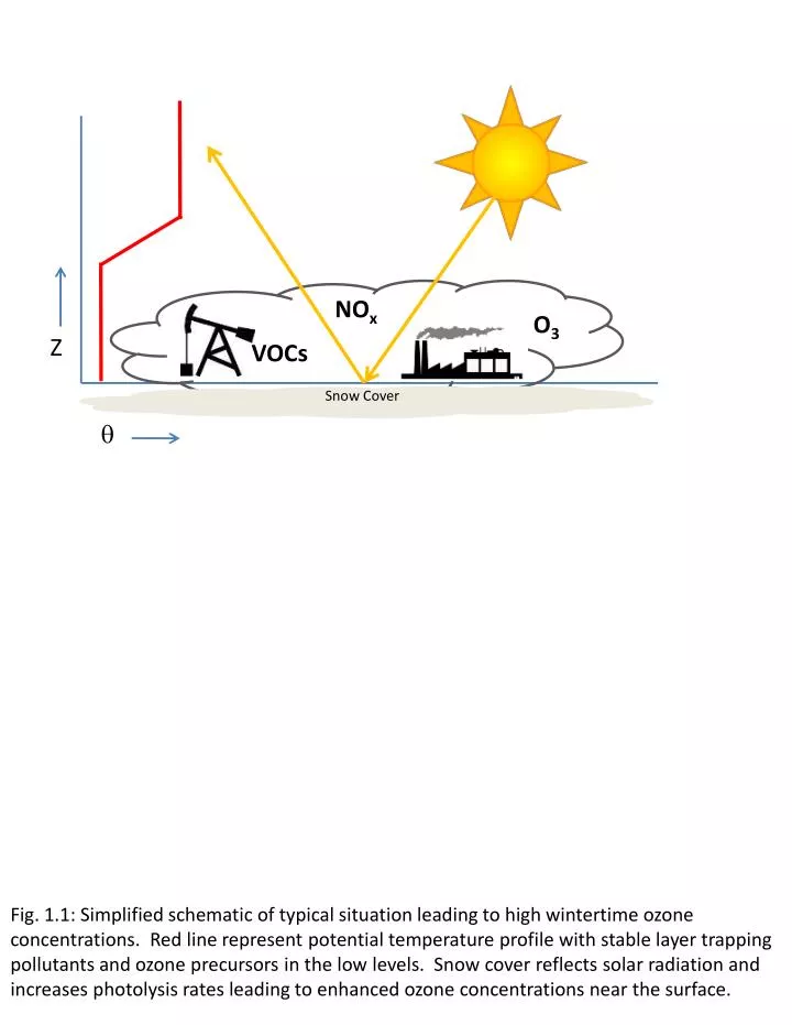
NOx VOCs O3 Snow Cover Z q Fig. 1.1: Simplified schematic of typical situation leading to high wintertime ozone concentrations. Red line represent potential temperature profile with stable layer trapping pollutants and ozone precursors in the low levels. Snow cover reflects solar radiationand increases photolysis rates leading to enhanced ozone concentrations near the surface.
(a) (b) (c) Fig. 1.2: Annual fossil fuel production in Uintah Basin since 2009 for (a) oiland (b) gas. (c) Total value of fossil fuel production in Utah since 2001. 1 barrel = 42 US gallons, 1 MCF = 1,000 cubic feet. Data provided by Utah Division of Oil, Gas, and Mining.
Fig. 1.3: Location of oil wells (green) and gas wells (red) operating inside the Uintah Basin in March 2014. Data provided by Utah Division of Oil, Gas, and Mining.
(a) (b) (c) Fig. 1.4: Satellite images showing examples of spatial snow cover variations in the Uintah Basin from the NASA SPoRT program’s snow-cloud product. Snow cover appears red, bare ground is cyan, and cloud cover is white. (a) Full snow cover on 2 Feb 2013, (b) snow melted in western portion of basin on 2 Feb 2014, and (c) no snow cover on basin floor on 21 Feb 2014.
4500 (a) 4000 3500 3000 2500 2000 1.33 km 4 km 1500 1000 500 12 km 0 4000 WY (b) 3750 3500 Uinta Mountains UT CO 3250 3000 VER ROO 2750 Wasatch Range RED 2500 MYT HOR OUR 2250 Tavaputs 2000 1750 Plateau 1500 Desolation Canyon 1250 Fig. 1.5: WRF 12-, 4-, and 1.33-km domains (a) with terrain contoured every 500 m. (b) Subdomain used for plotting with terrain contoured every 250 m and major geographic features labeled. Black dots indicate locations of MesoWest stations used for verification: Horsepool (HOR), Myton (MYT), Ouray (OUR), Red Wash (RED), Roosevelt (ROO), and Vernal (VER). Red line indicates position of vertical cross sections shown later in this paper.
Fig. 2.1: Surface observations inside the Uintah Basin at 1800 UTC on 2 February 2013. Dots represent station location and plotted values are air temperature (C). Red dots indicate locations used for model validation.
(b) (a) Fig. 2.2: WRF vertical model level setup. The bottom of model levels are plotted for (a) entire model domain (in km) and (b) lowest 2 km of domain (in m).
Fig. 2.3: Snow depth (blue) and snow water equivalent (red) as a function of elevation. Plotted values are from 0000 UTC on 1 Feb 2013 for Prescribed snow applied to WRF simulations (black line), observations (O) from the Uintah Basin and surrounding mountains, and NAM analysis (X). NAM analysis data was extracted along a southeast to northwest transect from the center of the basin to the center of the Uinta Mountains.
(a) (b) Fig. 2.4: WRF snow albedo field at 0100 UTC 01 Feb 2013 for (a) before and (b) after modifications to WRF snow albedo and VEGPARM.TBL. High albedos were attained in the Uintah Basin from the combination of edits to the WRF initial snow field, vegetation parameter table, and snow albedo. After these modifications, the Noah LSM produced albedo values within the basin in line with those measured by the Horsepool radiation suite.
(a) (b) (c) (d) 0 0.1 0.2 0.3 0.4 0.5 0.6 0.7 0.8 0.9 1 Fig. 2.5: Snow depth field from (a) NAM analysis at 0000 UTC 01 Feb 2013 and initialized snow depth field for (b) “Full Snow” case in BASE/FULL simulations, (c) “No Western Snow” case in NW simulation, and (d) “No Snow” case in NONE simulation.
5800 (a) 5700 5600 5500 5400 5300 5200 5100 5000 1025 (b) 1020 1015 1010 1005 1000 995 990 Fig. 3.0: NCEP North American Regional Reanalysis composite plots from 0000 UTC 1 February to 0000 UTC 7 February 2013 for (a) 500 hPageopotential height (in m) and (b) mean sea level pressure (in hPa).
(a) (b) (c) Fig. 3.1: Rawinsondes released from Roosevelt at (a) 1800 UTC 2 February 2013, (b) 1800 UTC 4 February 2013, and (c) 1800 UTC 6 February 2013. Temperature is in red and dewpoint is in blue. Wind barbs on right side denote wind speed and direction (full barb = 5 m s-1).
(a) (b) Fig. 3.2: VIIRS satellite imagery from NASA SPoRT program. (a) Nighttime Microphysics RGB product at 0931 UTC 2 Feb 2013 and (b) Snow-Cloud RGB product at 1815 UTC 2 Feb 2013.
(a) 4 km (b) Fig. 3.3: (a) Ozone concentrations from 1-10 February 2013 for Roosevelt (black), Horsepool (blue), Vernal (red), and Ouray (green). The NAAQS of 75 ppb (8-hour mean) is noted by the thin black dashed line. (b) Ceilometer backscatter (shaded) and estimated aerosol depth (black dots) at Roosevelt from 1 - 7 Feb 2013. Red colors indicate the presence of fog or clouds and unshaded regions indicate beam attenuation.
4 (a) 2 0 -2 -4 -6 -8 -10 -12 4 (b) 2 0 -2 -4 -6 -8 -10 -12 Fig. 3.4: 2-m Temperatures shaded every 0.5 °C at 1800 UTC 2 Feb 2013 for (a) BASE and (b) FULL simulations. Black contour indicates terrain elevation of 1800 m as a reference for Uintah Basin location.
Fig. 3.5: Time series of mean 2-m Temperature Bias for BASE (red), FULL (blue), NONE (red), and NW (magenta) simulations. Biases are averaged for the six surface stations in Fig. 1b.
(a) (b) (c) (d) (e) (f) Fig. 3.6: Potential temperature profiles at Roosevelt at 1800 UTC on (a) 1 Feb 2013, (b) 2 Feb 2013, (c) 3 Feb 2013, (d) 4 Feb 2013, (e) 5 Feb 2013, and (f) 6 Feb 2013. Profiles are shown for the observed sounding (dashed black), BASE (green), FULL (blue), NONE (red), and NW (magenta). On several plots, FULL (blue) is covered by NW (magenta) because the profiles are so similar.
3.0 3.0 (a) (b) 2.5 2.5 2.0 2.0 1.5 1.5 W E W E 3.0 3.0 (c) (d) 2.5 2.5 2.0 2.0 1.5 1.5 W E W E Fig. 3.7: Vertical cross sections of potential temperature (shaded every 1 K) and wind speed (contoured every 2.5 m s-1, bold and labeled every 5 m s-1), taken along red line in Fig. 1b. Results shown from BASE simulation for (a) 1800 UTC 1 Feb 2013, (b) 0600 UTC 3 Feb 2013, (c) 1800 UTC 4 Feb 2013 and (d) 1500 UTC 6 Feb 2013.
(a) BASE (b) FULL (c) NONE 2 7 4 3 1 5 6 Day of February Fig. 3.8: Time-height plot of potential temperature (shaded and contoured every 1 K) at Horsepool from 1 - 6 Feb 2013.
(a) 40 35 30 25 20 15 10 5 FRU STA LRF MYT OUR HOR ROO 3.0 (b) 304 302 300 298 2.5 296 294 292 Height (km) 290 288 2.0 286 284 282 280 278 1.5 276 50 200 100 150 W E Distance (km) Fig. 3.9: BASE simulation results at 0600 UTC 4 Feb 2013 for (a) 2.3km MSL wind speed (shaded every 2.5 m s-1) and barbs. (b) Vertical cross section of potential temperature (shaded every 1 K) along red line in Fig. 1b.
(b) (a) (d) (c) -2 0 -8 -12 -10 -6 -4 2 Fig. 3.10: Mean 2-m temperature (C) over entire 6-day simulation for (a) BASE, (b) FULL, (c) NW, (d) NONE.
(a) Difference In longwave Radiation from Clouds (W m-2) 20 15 10 5 0 2 (b) 2-m Temperature Difference (C) 1.5 1 0.5 0 -0.5 Fig. 3.11: (a) Average difference in downwelling longwave radiation (BASE - FULL) from 1 Feb 0000 UTC to 7 Feb 0000 UTC. Liquid clouds in BASE generally produced 10-20 Wm-2 more longwave radiation than ice clouds in FULL. (b) Average difference in 2-m temperatures (BASE - FULL) for the same period.
(a) Integrated Clouds (mm) (b) Integrated Clouds (mm) (c) Cloud Water (g kg-1) (d) Cloud Ice (g kg-1) (e) LW Radiation from Clouds (W m-2) (f) LW Radiation from Clouds (W m-2) Fig.3.12: Comparison of cloud characteristics between BASE (a,c,e) and FULL (b,d,f) model runs at 0600 UTC 5 Feb 2013. (a,b) Integrated cloud amount (c) mean cloud water in bottom 15 model levels, (d) mean cloud ice in bottom 15 model levels, (e,f) net downwellinglongwave radiation from clouds.
(a) (b) (c) (d) Fig. 3.13: Potential temperature profiles at Ouray on 3 Feb at (a) 0900 UTC, (b) 1200 UTC, (c) 1500 UTC, and (d) 1800 UTC for FULL (blue) and NONE (red). Tethersonde observations below 1700 m MSL at 1500 and 1800 UTC are shown for comparison.
Fig. 3.14: Mean zonal wind difference (m s-1) between NW and FULL simulations (NW-FULL). Results averaged over entire 6-day simulation. Thick black contour represents terrain elevation o f 1800 m, thin black contour represents region where snow is removed in the NW simulation.
(a) (b) Fig. 3.15: Time- and space-averaged zonal wind along cross-section in Fig. X over the entire simulation period for (a) FULL and (b) NONE. Westerly flow is filled red, easterly flow is filled blue. Westerly contours are every 2 m s-1, easterly contours are at -0.5, -1, and -2 m s-1. Values are averaged over a 26-km region perpendicular to the cross section with 10 grid points on each side of the centerline.
(a) (b) Fig. 3.16: Same as Fig. 3.15, but only daytime hours (0800 to 1700 local time) are included in the time-average.
(a) (b) Fig. 3.17: Same as Fig. 3.16, except for nighttime hours (1800 to 0700 local time).
(a) N NE NW E W (b) SW SW S N S N E W Fig. 3.18: Mean 10-m wind direction during (a) daytime periods (0800 to 1700 local time) and (b) nighttime periods (1800 to 0700 local time) for the FULL simulation.
(a) (b) Fig. 4.1 Ozone concentrations from mobile transect on 6 Feb 2013 from 1130 to 1500 Mountain Standard Time. (a) Spatial concentration
(a) FULL (b) NONE Fig. 4.2: Time-averaged ozone concentration (ppb) on lowest CMAQ model level (~17.5 m) for (a) FULL (b) NONE WRF simulations. Only mid- to late-day hours (1100 to 1700 local time) are included. Thin black line outlines region of greater than 75 ppb ozone concentration. Thick black line contours terrain elevation of 1800 m as a reference for Uintah Basin location.
Fig. 4.3: 4km model domain used in CMAQ simulations with terrain shaded and contoured every 500 m. The thick red line marks location of ozone cross sections in Fig. 4.4 and the thin red lines indicate spatial extent of area-average in direction perpendicular to cross section. The blue box represents the area used for mean shortwave radiation calculations in Fig. 4.7, and the green dot indicates location of Seven Sisters ozone monitoring station discussed in text.
(a) FULL (b) NONE Fig. 4.4: Time- and space-averaged ozone concentration along cross section in Fig. 1b for (a) FULL (b) NONE WRF simulations. Only mid- to late-day hours (1100 to 1700 local time) are included in time-average. Output from the 4-km domain was run through CMAQ to produce concentrations at 4-km resolution. Values are averaged over a 24-km region perpendicular to the cross section with 3 grid points on each side of the centerline.
(a) Roosevelt (b) Horsepool (c) Seven Sisters Fig. 4.5: Time Series of ozone concentrations for (a) Roosevelt, (b) Horsepool, and (c) Seven Sisters. Observations are in black, CMAQ output from FULL (NONE) is blue (red), and the NAAQS is noted by the thin black dashed line.
(a) FULL (b) NONE Day of February 7 7 4 4 3 3 2 2 1 1 5 5 6 6 Fig. 4.6: Time-height plot of potential temperature (shaded and thin black contours) and ozone concentrations (colored contours) for (a) FULL and (b) NONE simulations. Ozone concentrations are contoured every 10 ppb, starting at 75 ppb and alternate between solid and dashed every 10 ppb.
(a) Downward Shortwave (b) Upward Shortwave (b) Total Shortwave (Up + Down) Fig. 4.7: Time series of shortwave radiation data for FULL (blue), and NONE (red) simulations. (a) Downward radiation at the surface, (b) upward (reflected) radiation at the surface, and (c) Total radiation (Up + Down). Values are averaged over a 26 by 39 km box in the center of the basin (shown in Fig 4.3).
Table 3.1. 2-m temperature errors from WRF simulations. Mean errors calculated from the six surface stations in Fib 1b. Table 3.2. WRF simulation sensitivity to microphysics. Difference in longwave radiation and 2-m temperature between BASE and FULL simulations. Mean values shown for area below selected terrain contours within the basin. Table 3.3. 2-m temperature difference from FULL simulation
Table 4.1. Ozone statistics from CMAQ model forced by FULL and NONE simulations.