Download
1 / 35
360 likes | 548 Views
ISSUES IN BOUNDARY LAYER PARAMETRIZATION FOR LARGE SCALE MODELS Anton Beljaars* (ECMWF). Boundary layer clouds Wind turning Momentum budget (heterogeneous terrain). With contributions from: Andy Brown, Sylvain Cheinet, Hans Hersbach, Martin Koehler, Andrew Orr.

E N D
ISSUES IN BOUNDARY LAYER PARAMETRIZATION FOR LARGE SCALE MODELSAnton Beljaars*(ECMWF) • Boundary layer clouds • Wind turning • Momentum budget (heterogeneous terrain) • With contributions from: Andy Brown, Sylvain Cheinet, Hans Hersbach, Martin Koehler, Andrew Orr UCLA workshop June 2005
Recent implementation of Mass-flux/K-diffusion approach • key ingredients: • moist conserved variables • combined Mass-flux/K-diffusion solver • cloud variability • transition between stratocumulus and shallow convection UCLA workshop June 2005
Results: Low cloud cover (new-old) T511 time=10d n=140 2001 & 2004 old: CY28R4 new PBL UCLA workshop June 2005
Results: EPIC column extracted from 3D forecasts old PBL new MK PBL EPIC obs 700 750 800 850 900 950 1000 Liquid Water Path [g/m2] WV Mixing Ratio [g/kg] 300 45 250 200 Model Levels Pressure [hPa] 150 50 100 50 55 0 60 6 10 4 8 0 2 16 17 18 19 20 21 22 Local Time [October 2001 days] UCLA workshop June 2005
ARM SGP, number of cloudy hours in July 2003 Cloud radar Model Model lacks afternoon shallow cumulus Sylvain Cheinet (2005) UCLA workshop June 2005
ARM SGP, daily 36 hr back trajectories, July 2003 Cross section of model moisture and cloud cover for fair weather days in July 2003 (q: shaded; cc: contours at 0.01, 0.02, 0.05) L42, 600 hPa L54, 950 hPa UCLA workshop June 2005
ARM SGP, surface fluxes(model/obs) West-East change of LE/H Monthly domain averaged diurnal cycle LE H Time evolution of LE and H for station C1 UCLA workshop June 2005
ARM SGP, 2m T/q, BL wind (model/obs) 28R1 +MO stable BL 28R1 UCLA workshop June 2005
ARM SGP: Sensitivity to shallow convection Cross section of model humidity difference for fair weather days in July 2003 (Effect of halving shallow convection mass flux over land) Cross section of model humidity difference for fair weather days in July 2003 (Effect of No Shallow Convection) UCLA workshop June 2005
Boundary layer cloud issues • The switching algorithm is unsatisfactory. Unification between stratocumulus and shallow cumulus is desirable. What is the physical mechanism that controls the regime? • Numerics of inversion handling • Cloud top entrainment? • Closure for shallow convection? • Does a scheme have the correct feedbacks and how can we test this? • What is the role of shallow convection in more complicated situations (cold air outflow, momentum transport) UCLA workshop June 2005
Geostrophic drag law Wangara data drag a-geostrophic angle UCLA workshop June 2005
Operational verification of surface wind A-geostrophic angle is too small UCLA workshop June 2005
Operational verification of surface wind Wind speed is too low during the day and too high at night UCLA workshop June 2005
Examples of ERA40 forecast veers Brown et al. 2005 20020213 12Z+24 20020214 12Z+24 250m T and wind Surface to 850 hPa veer >27o 12o27o -12o12o -27o-12o <-27o Backing on and behind cold front Veering in warm sector of depression UCLA workshop June 2005
Atlantic sonde stations • SST, December 1987 MIKE LIMA CHARLIE SABLE UCLA workshop June 2005
Veering between surface (10m) and 850 hPa wind: comparison of 24 hour ERA40 forecast with 12Z sonde UCLA workshop June 2005
Composite ERA40 results(4 winters; Sable, Charlie, Lima and Mike combined) • When sonde shows big veering, model veers less • When model shows big veering, sonde veers more • Model definitely under-veers • When sonde shows big backing, model backs less • When model shows big backing, sonde veers are similar • Model probably under-backs UCLA workshop June 2005
Errors in ERA40 surface wind direction as f (surface wind direction) • Southerly flow at Sable and Charlie likely to be associated with warm advection • Insufficient turning across boundary layer • Forecast surface wind veered relative to observed wind • Northerly flow at Sable and Charlie likely to be associated with cold advection • Forecast wind direction errors become small, and possibly reverse (lack of backing across boundary layer) • Possible that plotting versus wind direction is not selective enough to pick out the strongest cold advection cases where lack of backing is most likely UCLA workshop June 2005
Impact of resolution and model • Qualitatively similar results in ECMWF T511 operational model and also in Met Office operational model UCLA workshop June 2005
Stable boundary layer diffusion Diffusion coefficients based on Monin Obukhov similarity: UCLA workshop June 2005
Impact of MOSBL on veers (1 winter; Sable, Charlie, Lima and Mike combined) • Typically increased 5o in stable cases • Further weakening of mixing by reducing length scale from 150m to 50m gives further small increase UCLA workshop June 2005
Wind direction from QuikSCAT UCLA workshop June 2005
Wind direction • Operational models underestimate a-geostrophic angle (what controls boundary layer veering?) • Stable boundary layers do occur frequently over the ocean • Real boundary layers are baroclinic (systematic LES simulations covering a wide range of baroclinicity may be helpful?) UCLA workshop June 2005
Surface drag, momentum budget • Surface drag is controlled by boundary layer mixing and surface roughness length • Less boundary layer mixing (e.g. in stable boundary layer) leads to less surface drag • Surface drag (or effective roughness) over land is very uncertain due to terrain heterogeneity effects UCLA workshop June 2005
Z0-table UCLA workshop June 2005
z0 UCLA workshop June 2005
CD-control UCLA workshop June 2005
TOD+new z0 table UCLA workshop June 2005
MO UCLA workshop June 2005
Zonal mean West-East turb. stress ZM stress + Ps Zonal mean surf. press. error (step=24) Control New z0-table Control New z0-table Control MO-stab.f. Control MO-stab.f. UCLA workshop June 2005
Error tracking Control MO-stab.f. UCLA workshop June 2005
500 hPa RMSerror NH, 200403 Control MO-stab.f. 500 hPa activityDivided byAnalysis activity NH, 200403 Control MO-stab.f. UCLA workshop June 2005
500 hPa RMSerror NH, 200403 Control New z0-table 500 hPa activityDivided byAnalysis activity NH, 200403 Control New z0-table UCLA workshop June 2005
BL-Veering Control Control-New z0-table Control-MO UCLA workshop June 2005
Conclusions • NWP is sensitive to surface drag. Drag is affected by vegetation roughness, orographic effects and stability. • It is difficult to verify surface drag. • Roughness lengths are derived from land use data sets, without considering heterogeneity. Results are uncertain. Research topics • Derive geometric land use parameters from satellite data • Run high resolution canopy resolving models to “measure” effective roughness length and its interaction with stability • Infer surface drag from synoptic development (variational techniques that minimize short range forecast errors?) UCLA workshop June 2005