Support Vector Machines

Support Vector Machines MEDINFO 2004, T02: Machine Learning Methods for Decision Support and Discovery Constantin F. Aliferis & Ioannis Tsamardinos Discovery Systems Laboratory Department of Biomedical Informatics Vanderbilt University

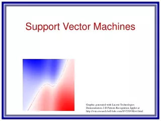
Support Vector Machines • Decision surface is a hyperplane (line in 2D) in feature space (similar to the Perceptron) • Arguably, the most important recent discovery in machine learning • In a nutshell: • map the data to a predetermined very high-dimensional space via a kernel function • Find the hyperplane that maximizes the margin between the two classes • If data are not separable find the hyperplane that maximizes the margin and minimizes the (a weighted average of the) misclassifications

Support Vector Machines • Three main ideas: • Define what an optimal hyperplane is (in way that can be identified in a computationally efficient way): maximize margin • Extend the above definition for non-linearly separable problems: have a penalty term for misclassifications • Map data to high dimensional space where it is easier to classify with linear decision surfaces: reformulate problem so that data is mapped implicitly to this space

Which Separating Hyperplane to Use? Var1 Var2

Maximizing the Margin Var1 IDEA 1: Select the separating hyperplane that maximizes the margin! Margin Width Margin Width Var2

Why Maximize the Margin? • Intuitively this feels safest. • It seems to be the most robust to the estimation of the decision boundary. • LOOCV is easy since the model isimmune to removal of any nonsupport-vector datapoints. • Theory suggests (using VCdimension) that is related to (but notthe same as) the proposition that thisis a good thing. • It works very well empirically.

Why Maximize the Margin? • Perceptron convergence theorem (Novikoff 1962): • Let s be the smallest radius of a (hyper)sphere enclosing the data. • Suppose there is a w that separates the data, i.e., wx>0 for all x with class 1 and wx<0 for all x with class -1. • Let m be the separation margin of the data • Let learning rate be 0.5 for the learning rule • Then, the number of updates made by the perceptron learning algorithm on the data is at most (s/m)2

Support Vectors Var1 Support Vectors Margin Width Var2

Setting Up the Optimization Problem Var1 The width of the margin is: So, the problem is: Var2

Setting Up the Optimization Problem Var1 There is a scale and unit for data so that k=1. Then problem becomes: Var2

Setting Up the Optimization Problem • If class 1 corresponds to 1 and class 2 corresponds to -1, we can rewrite • as • So the problem becomes: or

Linear, Hard-Margin SVM Formulation • Find w,b that solves • Problem is convex so, there is a unique global minimum value (when feasible) • There is also a unique minimizer, i.e. weight and b value that provides the minimum • Non-solvable if the data is not linearly separable

Solving Linear, Hard-Margin SVM • Quadratic Programming • QP is a well-studied class of optimization algorithms to maximize a quadratic function of some real-valued variables subject to linear constraints. • Very efficient computationally with modern constraint optimization engines (handles thousands of constraints and training instances).

Non-Linearly Separable Data Var1 Find hyperplane that minimize both ||w|| and the number of misclassifications: ||w||+C*#errors Problem: NP-complete Plus, all errors are treated the same Var2

Non-Linearly Separable Data Var1 Minimize ||w||+C*{distance of error points from their desired place} Allow some instances to fall within the margin, but penalize them Var2

Non-Linearly Separable Data Var1 Introduce slack variables Allow some instances to fall within the margin, but penalize them Var2

Formulating the Optimization Problem Constraints becomes : Objective function penalizes for misclassified instances and those within the margin C trades-off margin width and misclassifications Var1 Var2

Linear, Soft-Margin SVMs • Algorithm tries to maintain i to zero while maximizing margin • Notice: algorithm does not minimize the number of misclassifications (NP-complete problem) but the sum of distances from the margin hyperplanes • Other formulations use i2 instead • As C, we get closer to the hard-margin solution • Hard-margin decision variables = m+1, #constraints = n • Soft-margin decision variables = m+1+n, #constraints=2n

Var1 i Var2 Robustness of Soft vs Hard Margin SVMs Var1 Var2 Hard Margin SVN Soft Margin SVN

Soft vs Hard Margin SVM • Soft-Margin always have a solution • Soft-Margin is more robust to outliers • Smoother surfaces (in the non-linear case) • Hard-Margin does not require to guess the cost parameter (requires no parameters at all)

Var1 Var2 Disadvantages of Linear Decision Surfaces

Var1 Var2 Advantages of Non-Linear Surfaces

Linear Classifiers in High-Dimensional Spaces Constructed Feature 2 Var1 Var2 Constructed Feature 1 Find function (x) to map to a different space

Mapping Data to a High-Dimensional Space • Find function (x) to map to a different space, then SVM formulation becomes: • Data appear as (x), weights w are now weights in the new space • Explicit mapping expensive if (x) is very high dimensional • Solving the problem without explicitly mapping the data is desirable

The Dual of the SVM Formulation • Original SVM formulation • n inequality constraints • n positivity constraints • n number of  variables • The (Wolfe) dual of this problem • one equality constraint • n positivity constraints • n number of  variables (Lagrange multipliers) • Objective function more complicated • NOTICE: Data only appear as (xi)  (xj)

The Kernel Trick • (xi)  (xj): means, map data into new space, then take the inner product of the new vectors • We can find a function such that: K(xi  xj) = (xi)  (xj), i.e., the image of the inner product of the data is the inner product of the images of the data • Then, we do not need to explicitly map the data into the high-dimensional space to solve the optimization problem (for training) • How do we classify without explicitly mapping the new instances? Turns out

Examples of Kernels • Assume we measure two quantities, e.g. expression level of genes TrkC and SonicHedghog (SH) and we use the mapping: • Consider the function: • We can verify that:

Polynomial and Gaussian Kernels • is called the polynomial kernel of degree p. • For p=2, if we measure 7,000 genes using the kernel once means calculating a summation product with 7,000 terms then taking the square of this number • Mapping explicitly to the high-dimensional space means calculating approximately 50,000,000 new features for both training instances, then taking the inner product of that (another 50,000,000 terms to sum) • In general, using the Kernel trick provides huge computational savings over explicit mapping! • Another commonly used Kernel is the Gaussian (maps to a dimensional space with number of dimensions equal to the number of training cases):

The Mercer Condition • Is there a mapping (x) for any symmetric function K(x,z)? No • The SVM dual formulation requires calculation K(xi , xj) for each pair of training instances. The array Gij = K(xi , xj) is called the Gram matrix • There is a feature space (x) when the Kernel is such that Gis always semi-positive definite (Mercer condition)

Other Types of Kernel Methods • SVMs that perform regression • SVMs that perform clustering • -Support Vector Machines: maximize margin while bounding the number of margin errors • Leave One Out Machines: minimize the bound of the leave-one-out error • SVM formulations that take into consideration difference in cost of misclassification for the different classes • Kernels suitable for sequences of strings, or other specialized kernels

Variable Selection with SVMs • Recursive Feature Elimination • Train a linear SVM • Remove the variables with the lowest weights (those variables affect classification the least), e.g., remove the lowest 50% of variables • Retrain the SVM with remaining variables and repeat until classification is reduced • Very successful • Other formulations exist where minimizing the number of variables is folded into the optimization problem • Similar algorithm exist for non-linear SVMs • Some of the best and most efficient variable selection methods

Neural Networks Hidden Layers map to lower dimensional spaces Search space has multiple local minima Training is expensive Classification extremely efficient Requires number of hidden units and layers Very good accuracy in typical domains SVMs Kernel maps to a very-high dimensional space Search space has a unique minimum Training is extremely efficient Classification extremely efficient Kernel and cost the two parameters to select Very good accuracy in typical domains Extremely robust Comparison with Neural Networks

Why do SVMs Generalize? • Even though they map to a very high-dimensional space • They have a very strong bias in that space • The solution has to be a linear combination of the training instances • Large theory on Structural Risk Minimization providing bounds on the error of an SVM • Typically the error bounds too loose to be of practical use

MultiClass SVMs • One-versus-all • Train n binary classifiers, one for each class against all other classes. • Predicted class is the class of the most confident classifier • One-versus-one • Train n(n-1)/2 classifiers, each discriminating between a pair of classes • Several strategies for selecting the final classification based on the output of the binary SVMs • Truly MultiClass SVMs • Generalize the SVM formulation to multiple categories • More on that in the nominated for the student paper award: “Methods for Multi-Category Cancer Diagnosis from Gene Expression Data: A Comprehensive Evaluation to Inform Decision Support System Development”, Alexander Statnikov, Constantin F. Aliferis, Ioannis Tsamardinos

Conclusions • SVMs express learning as a mathematical program taking advantage of the rich theory in optimization • SVM uses the kernel trick to map indirectly to extremely high dimensional spaces • SVMs extremely successful, robust, efficient, and versatile while there are good theoretical indications as to why they generalize well

Suggested Further Reading • http://www.kernel-machines.org/tutorial.html • C. J. C. Burges. A Tutorial on Support Vector Machines for Pattern Recognition. Knowledge Discovery and Data Mining, 2(2), 1998. • P.H. Chen, C.-J. Lin, and B. Schölkopf. A tutorial on nu -support vector machines. 2003. • N. Cristianini. ICML'01 tutorial, 2001. • K.-R. Müller, S. Mika, G. Rätsch, K. Tsuda, and B. Schölkopf. An introduction to kernel-based learning algorithms. IEEE Neural Networks, 12(2):181-201, May 2001. (PDF) • B. Schölkopf. SVM and kernel methods, 2001. Tutorial given at the NIPS Conference. • Hastie, Tibshirani, Friedman, The Elements of Statistical Learning, Springel 2001

Support Vector Machines