Download
1 / 24
240 likes | 439 Views
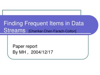
Finding Frequent Items in Data Streams [Charikar-Chen-Farach-Colton]. Paper report By MH , 2004/12/17. Finding Frequent Items in Data Streams. Today Synopsis Data Structures Sketches and Frequency Moments Finding Frequency Items in Data Streams. Synopsis Data Structures.

E N D
Finding Frequent Items in Data Streams [Charikar-Chen-Farach-Colton] Paper report By MH , 2004/12/17
Finding Frequent Items in Data Streams • Today • Synopsis Data Structures • Sketches and Frequency Moments • Finding Frequency Items in Data Streams
Synopsis Data Structures • Synopsis Data Structures • “Lossy” Summary (of a data stream) • Advantages – fits in memory + easy to communicate • Disadvantage – lossiness implies approximation error • Key Techniques – randomization and hashing
Random Samples • Goal maintain uniform sample of item-stream • Sampling Semantics? • Coin flip • select each item with probability p • easy to maintain • undesirable – sample size is unbounded • Fixed-size sample without replacement • Our focus today • Fixed-size sample with replacement • Show – can generate from previous sample • Non-Uniform Samples[Chaudhuri-Motwani-Narasayya]
2 2 1 1 1 m0 m1 m2 m3 m4 Data stream: 2, 0, 1, 3, 1, 2, 4, . . . Generalized Stream Model • Input Element(i,a) • a copies of domain-value i • increment to ith dimension of m by a • a need not be an integer
2 2 1 1 1 m0 m1 m2 m3 m4 On seeing element (i,a) = (2,2) On seeing element (i,a) = (1,-1) 4 2 1 1 1 m0 m1 m2 m3 m4 Example 4 1 1 1 1 m0 m1 m2 m3 m4
Frequency Moments • Input Stream • values from U = {0,1,…,N-1} • frequency vector m = (m0,m1,…,mN-1) • Kth Frequency MomentFk(m) = Σi mik • F0: number of distinct values • F1: stream size • F2: Gini index, self-join size, Euclidean norm • Fk:for k>2, measures skew, sometimes useful • F∞: maximum frequency
Finding Frequent Items in Data Streams • Introduction • Main Idea • COUNT SKETCH Algorithm • Final result
Problem - This work was done while the author was at Google Inc. The Google Problem Return list of k most frequent items in stream Motivation search engine queries, network traffic, … Remember Saw lower bound recently! Solution Data structure Count-Sketch maintaining count-estimates of high-frequency elements
Introduction (1) • One of the most basic problems on a data stream [HRR98,AMS99] is that of finding the most frequently occurring items in the stream • We shall assume here that the stream is large enough that memory-intensive solutions such as sorting the stream or keeping a counter for each distinct element are infeasible • This problem comes up in the context of search engines, where the streams in question are streams of queries sent to the search engine and we are interested in finding the most frequent queries handled in some period of time.
Introduction (2) • A wide variety of heuristics for this problem have been proposed, all involving some combination of sampling, hashing, and counting (see [GM99] and Section 2 for a survey). • However, none of these solutions have clean bounds on the amount of space necessary to produce good approximate lists of the most frequent items.
Definitions • Notation • Assume {1, 2, …, N} in order of frequency • miis frequency of ith most frequent element • m = Σmiis number of elements in stream Two notions of approximating the frequent-element problem • FindCandidateTop • Input: stream S, int k, int p • Output: list of p elements containing top k • FindApproxTop • Input: stream S, int k, real • Output: list of k elements, each of frequency mi > (1-) mk
FindCandidateTop • for example, that nk = np+1 + 1, that is, the k-th most frequent element has almost the same frequency as the p + 1st most frequent element. Then it would be almost impossible to find only p elements that are likely to have the top k elements. • We therefore define the following variant: FindApproxTop
Main Idea • Consider • single counter X • hash function h(i): {1, 2,…,N}{-1,+1} • Input element i update counter X += Zi = h(i) • For each r, use XZr as estimator of mr Theorem:E[XZr] = mr Proof • X = Σi miZi • E[XZr] = E[Σi miZiZr] = Σi miE[Zi Zr] = mrE[Zr2] = mr
A couple of problems • The variance of every estimate is very large • O(N) elements have estimates that are wrong by more than the variance.
Array of Counters • Idea – t counters,c1,...ct, t hash function h1,…,ht • We can then take the mean or median of these estimates to achieve an estimate with lower variance.
Problem with “Array of Counters” • Variance – dominated by highest frequency • Estimates for less-frequent elements like k • corrupted by higher frequencies • Avoiding Collisions? • spread out high frequency elements • replace each counter with hashtable of b counters
s1 : i {1, ..., b} h1: i {+1, -1} st : i {1, ..., b} ht: i {+1, -1} Count Sketch data structure • Hash Functions • independent hashes h1,...,htand s1,…,st • hashes independent of each other • Data structure: hashtables of counters X(r,c) 1 2 … b
configuration and operations • sr(i) – one of b counters in rth hashtable • ADD(i): for each r, update X(r,sr(i)) += hr(i) • Estimator(mi) = medianr { X(r,sr(i)) • hr(i) } • Maintain heap of k top elements seen so far
Why we choose median • we have not eliminated the problem of collisions with high-frequency elements, and these will still spoil some subset of the estimates. The mean is very sensitive to outliers, while the median is sufficiently robust.
Overall Algorithm • 1. Add(i) • 2. If i is in the heap, increment its count. Else, add i to the heap if Estimate(mi) is greater than the smallest estimated count in the heap. • In this case, the smallest estimated count should be evicted from the heap. • This algorithm solves FindApproxTop where our choice of b will depend on . • we can add and subtract . Thealgorithm takes space O(tb + k).And we bound t and b.
Final Results (1) • bound t and b • t =O(log m/) , where the algorithm fails with probability at most • b = O(k + i>k mi2 / (mk)2) (5 lemmas and 1 theorem are listed in the rear) • So…..
Final Results (2) • FindApproxTop • O([k + (i>kmi2) / (mk)2] log m/) • Zipfian Distribution:mi 1/i • gives improved results • compare with Sampling algorithm. • Finding items with largest frequency change • This problem also has a practical motivation in the context of search • engine query streams, since the queries whose frequency changes • most between two consecutive time periods can indicate which • topics people are currently most interested in [Goo].
5 Lemmas and 1 theorem(1) • nq(l) be the number of occurrences of element q up to position l. • Ai[q] be the set of elements that hash onto the same bucket in the i-th row as q does