Download
1 / 32
330 likes | 647 Views
THE PENDULUM AS A PERTURBED ROTOR. By Emmanuel N Nenghabi Coordinated by Prof.Charles Myles. OVERVIEW OF PRESENTATION. INTRODUCTION TO CANONICAL PERTURBATION THEORY LIE TRANSFORMS PERTURBATION THEORY WITH LIE SERIES THE PENDULUM AS A PERTURBED ROTOR USING LIE GENERATOR OBSERVATION

E N D
THE PENDULUM AS A PERTURBED ROTOR By Emmanuel N Nenghabi Coordinated by Prof.Charles Myles
OVERVIEW OF PRESENTATION • INTRODUCTION TO CANONICAL PERTURBATION THEORY • LIE TRANSFORMS • PERTURBATION THEORY WITH LIE SERIES • THE PENDULUM AS A PERTURBED ROTOR USING LIE GENERATOR • OBSERVATION • CONCLUSION
INTRODUCTION TO CANONICAL PERTURBATION THEORY • Closed form solutions of dynamical systems can rarely be found. • Examples-the two and three body problems in central force motion. Thus there is the need for an approximate solution. • The goal of perturbation theory is to relate aspects of the motion of the system to those of the nearby solvable system. The more complicated problem is then said to be a perturbation of the solubleproblem and the difference between the Hamiltonians is called the perturbation Hamiltonian.
INTRODUCTION TO CANONICAL PERTURBATION THEORY • The goal is to find a way to transform the exact solution of this approximate problem into an approximate solution of the original problem. • We can use the perturbation to try to predict the qualitative features of the solution by describing the characteristics ways in which the solutions of the solvable system are distorted by the additional effects. For instance, we might one to predict where the largest resonance regions are located or the locations and sizes of the largest chaotic zones. Being able to predict such features can give an insight into the behavior of the particular system of interest.
INTRODUCTION TO CANONICAL PERTURBATION THEORY • Suppose we have a system characterized by a Hamiltonian that breaks up into parts: H = H0 + εH1 where H0 is solvable and ε is a small parameter. The difference between our system and a solvable system is the small additive complication.
INTRODUCTION TO CANONICAL PERTURBATION THEORY • There are number of strategies for doing this. One strategy is to seek a canonical transformation that eliminates from the Hamiltonian the terms of order ε that impede the solution-this typically introduces terms of order ε2. Then one seeks another transformation that eliminates the terms of order ε2, impeding the solution leaving terms of order ε3. • We can imagine repeating this process until the part that impedes is of such high order of ε that it can be neglected. Having reduced the problem to a solvable problem, we can reverse the sequence of transformation to find an approximate solution of the original problem.
INTRODUCTION TO CANONICAL PERTURBATION THEORY • Does this process converge? How do we know we can ever neglect the remaining terms? • Classical perturbation theory has two classes- time dependent and time independent perturbation theory. We will follow the time dependent perturbation theory in this presentation
PERTURBATION THEORY WITH LIE SERIES • Given a physical system, we look for the decomposition of the Hamiltonian in the form: • H(t,p,q )= H0(t,p,q) + εH1(t,p,q) ……………………………….(1) where H0(t,p,q) represents the Hamiltonian for the soluble unperturbed problem. Some of the assumptions made are: • The Hamiltonian has no explicit time dependence • The Canonical Transformation has been made so that H0 depends only on the momenta i.e. this solution has been obtained from a Canonical Transformation in which the new Hamiltonian, H0, for the unperturbed problem is zero. • We carry out a Lie transformation and find the solutions that the Lie generator W must satisfy to eliminate the terms of order ε from the Hamiltonian.
LIE TRANSFORMS • Definition: A Lie transform, W, is a canonical transformation generated by another Hamiltonian like function in the same phase space i.e. E’ε,w of a function F of phase space coordinates (t, p,q) is defined by: E’ε,wF = FC’ε,w where E’ε,wF is the Lie transform of the function F.
PROPERTIES OF LIE TRANSFORMS • In terms of E’ε,w we have the canonical transformation: • p = (E’ε,wP)(t,q’,p’) • q = (E’ε,wQ)(t,q’,p’) • H’ = E’ε,wH • The identity function I = E’0,w and the Inverse function (E’ε,w)-1 = E’-ε,w
LIE SERIES • Taylor’s theorem gives us a way of approximating the value of a nice enough function at a point to a point where the value is known. If we know f and all of its derivatives at t then we can get the value of f(t+ε), for small enough ε as follows: • f(t+ε)= f(t)+εDf(t)+ 1/2ε2D2f(t) +… • This suggests that we can formally construct a Taylor series operator as the exponential of a differential operator: • eεD = I+ εDf(t) +1/2(εD)2f(t) +…… and write: • f(t+ε) =(eεDf)(t), where D is the differential operator.
LIE TRANSFORMS • The lie transform and associated Lie series specify a canonical transformation: • H’=E’εwH= e εLwH • q=(E’εwQ)(t,q’,p’) =(Q)(t’,q’,p’) • p=(E’εwP)(t,q’,p’) =(P)(t’,q’,p’) • (t,q,p) = (E’εwI)(t,q’,p’) =(I)(t,q’,p’)……………(2) where I is the identity function. By definition: • e εLwF = F + εLwF + ½ ε2L2WF +… = F + ε{F,W} + ½ ε2{F,W},W} +… with LwF ={F,W} • Applying the Lie transform to equation (1) we get:
LIE TRANSFORMS • H’ = eεLwH = H0 + εLwH0 +1/2ε2L2wH0 +. + εH1 + ε2L2wH1+…. =H0 + ε(LwH0+H1) + ε2(1/2LwH0 +LwH1) +… • The first order term in ε is zero if LwH0+H1=0, which is a linear partial differential equation for W. The transformed Hamiltonian is : • H’ = H0 + ε2(1/2L2wH0 + LwH1)+ .. = H0 + 1/2 ε2LwH1+…. Because 1/2ε2Lw{ LwH0 + H1+ H1}= 1/2 ε2LwH1
LIE TRANSFORMS • Thus we have eliminated terms of order ε but generated new terms of order ε2 and higher. • At this point, we can find an approximate solution by truncating the Hamiltonian equation in equation (1) to H0 which is soluble. The approximate solution for a given initial conditions (t0, q0, p0) is obtained by finding the corresponding (t0,q0’,p0’) using the inverse transformation given by equation (2). Then the system is evolved to time t using the solutions of the truncated Hamiltonian H0, giving the state (t, q’,p’). The phase coordinate of the evolved point are transformed back to the original variables in equation (2) to state (t,q,p).
THE PENDULUM AS A PERTURBED ROTOR • The pendulum is a simple one degree of freedom system for which the solutions are known. • For small displacements, the pendulum behaves like a simple harmonic oscillator and is isochronous i.e. the frequency is independent of amplitude. As the amplitude increases, the potential energy deviates from the harmonic oscillator form and the frequency shows a small dependence on the amplitude. The small difference between the potential energy and the harmonic oscillator limit can be considered as the perturbation Hamiltonian.
THE PENDULUM AS A PERTURBED ROTOR • The motion of a pendulum consisting of a mass point m at the end of a weightless rod of length l is: • H (t,θ,p) = 1/2mlθ2 +mgl(1-cosθ) where p=mlθ2 is the conjugate momentum • =p2/(2ml2) +mgl(1-cosθ) • = p2/2α –εβcosθ, where α=ml2, β=mgl • The parameter ε allows us to scale the perturbation (ε=1 for the actual pendulum)
THE PENDULUM AS A PERTURBED ROTOR • The Lie generator that satisfies {H0,W} + H1=0 is:
THE PENDULUM AS A PERTURBED ROTOR • The transformedHamiltonian is H’ = H0 + O(ε2). • If terms of O(ε2) can be ignored, then the transformed Hamiltonian is simple: • H’(t, θ’,p’) = p’2/2α with solutions:
THE PENDULUM AS A PERTURBED ROTOR To connect these solutions to the solutions of the original problem, we use the Lie series:
THE PENDULUM AS A PERTURBED ROTOR • Similarly • The time evolution of the system is defined by:
OBSERVATION • As the number of terms in the Lie series for the phase space coordination transformation increases, the results appear to converge. In fact terms of 2nd and higher orders of ε are closely clustered in one region of the phase space diagram
OBSERVATION • However, the behavior of the perturbative solution inside the oscillatory region is not like the real solution and does not converge. This is because it is assumed the real motion is a distorted version of the motion of the free rotor. In this region, this assumption is false (fig 2)
RANGE OF VALIDITY OF PERTURBATIVE SOLUTION(CRUDE ESTIMATE) • Let’s look at the first order correction term in: • This is not a small perturbation if
RANGE OF VALIDITY OF PERTURBATIVE SOLUTION(CRUDE ESTIMATE • The last equation scales for the validity of the perturbative solution. When H(t,θ=π,p)=εβ, the separatrix has a maximum momentum, pmax at θ=0. Thus H(t,π ,pmax) = H(t,π ,0). Note that pmax is half the width of the oscillatory region, i.e. • pmax=
RANGE OF VALIDITY OF PERTURBATIVE SOLUTION(CRUDE ESTIMATE • However the range of the perturbative solution can be improved by carrying out additional perturbation steps
HIGHER ORDER TERMS • After the first step, the Hamiltonian is, to the second order in ε,is given by: • H’(t,θ’,p’) = =H0(p’) + ε2H2(t,θ’,p’)
HIGHER ORDER TERMS • Performing a Lie transformation with the generator W’ yields: • H’’ = H0 + ε2(Lw’H0 + H2) +….. • The condition on W’ that the second order terms are eliminated is: • Lw’H0 + H2 =0 to get:
HIGHER ORDER TERMS • The new Lie generator W’
HIGHER ORDER TERMS • This solution is valid only for small time scales. For larger time scales the perturbative solution wanders all over the place as shown • The phase space coordinate transformation is obtained by carrying out the inverse transformation corresponding to W, then that for W’, solve the evolution of the system using H0, then transform back using W’ and the W. The approximate solution is shown pictorially
CONCLUSION • What the perturbation theory does is deforming the phase space coordinate system so that the problem looks like the free rotor problem. This works only for circular orbits. The perturbation theory works excellently outside the oscillatory region. The range of p in which the perturbation theory is not valid scales in the same way as the width of the oscillatory region. This need not have been the case; the perturbation theory would have failed over a wider region
REMARK • Having treated the motion of the moon about the earth, and having obtained an elliptical orbit, [Newton], considered the effect of the sun on the moon’s orbit by taking into account the variations of the latter. However, the calculations caused him great difficulties... Indeed, the problems he encountered were such that [Newton] was prompted to remark to the Astronomer John Machin that “…his head never ached but with his studies on the moon”_ June Barrow Green, Poincare and the three body problem [7], p15
BIBLIGRAPHY • Goldstein, Poole and Safko, Classical Mechanics 3rd ed., Addison Wesley 2001 • T. Thornton and B. Marion, Classical dynamics of particles and systems, 5th ed., Thomson-Brooks/Cole • Tai L. Chow, Classical Mechanics, John Wiley & Sons, Inc 1995 • B. Arfken and J. Weber, Mathematical Methods for Physicists, 4th ed.,Academic press • MIT PRESS ( www.press.mit.edu).