Download
1 / 25
310 likes | 706 Views
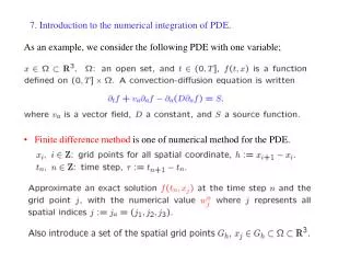
7. Introduction to the numerical integration of PDE. As an example, we consider the following PDE with one variable;. Finite difference method is one of numerical method for the PDE. Accuracy requirements. Usually t is more restricted by stability than by accuracy.

E N D
7. Introduction to the numerical integration of PDE. As an example, we consider the following PDE with one variable; • Finite difference method is one of numerical method for the PDE.
Accuracy requirements Usually t is more restricted by stability than by accuracy. Notation for the discretization of
Summary of the key concept on numerical method for PDE. • Local truncation error : The amount that the exact solution of PDE fails to • satisfy the the finite difference equation. • ex.) One-step method. • Global discretization error • Definitions: (Consistency) • Definitions: (Convergence)
Definitions: (Zero-Stability - a stability criteria with h ! 0 ) • Definitions: (Absolute Stability - a stability criteria with a fixed h) • Remark: Purpose of stability analysis is to determine t0(h) which guarantee that the perturbation does not glow. This is the case if • Note that for the case of Zero-stability, the dimension (size) of the matrix C0(h) increase as n !1 .
lp norm and l1 norm are defined by • Theorem: (Lax’s equivalence theorem) • Convergence ) Zero (or Absolute) - stability. • Zero (or Absolute) - stability and Consistency ) Convergence.
Some explicit integration method for a linear wave equation. • Some basic schemes for are presented. (1) FTCS (Forward in Time and Central difference Scheme). (2) Lax (- Friedrich) scheme. (3) Leap-Flog scheme (4) Lax-Wendroff scheme (5) 1st order upwind scheme
Some explicit integration method for a linear wave equation continued. • Lax, Lax-Wendroff, 1st order upwind schemes can be understood as • FTCS scheme +.Diffusion term. (1) Explicit Euler scheme (FTCS : Forward in Time and Central difference). (2) Lax (- Friedrich) scheme. (3) Lax-Wendroff scheme. (4) 1st order upwind scheme (weakest diffusion) (Can be used also for negative c.)
von Neumann stability analysis. • A method to analyze the stability of numerical scheme for linear PDE • (assuming equally spaced grid points and periodic boundary condition). • Consider that the finite difference equation has the following solution. • Then the perturbation can be also written Substituting the Fourier transform above, we have Amplification factor g(q) is defined by
The von Neumann condition for zero stability: The von Neumann condition for absolute stability:
Another derivation of von Neumann stability condition. Then we apply absolute stability condition for the ODE. Recall: • Test problem: • Characteristic polynomial Q: • Definition: The region of absolute stability for a one-step method is the set • Therefore for the PDE, the region of absolute stability is the set Note l2 norm. Parceval’s theorem.
Characteristic polynomials for a particular FD scheme. A substitution of to a FD equation, and the mode decomposition results in a equation for each Fourier component . Then, substituting we have characteristic polynomials. • A solution to the polynomial becomes an amplification factor for each mode q. • If the exact values are known, • conveniently shows amplification rate and • phase error of each mode. • Note: q = 0, corresponds to low frequency (long wavelength). • q = p, corresponds to high frequency (short wavelength).
Finite volume discretization Another concept for deriving finite difference approximation suitable for the conservation law; PDEs of the conservative form j–1/2 j+1/2 j–1 j j+1 unit volume Define a flux at the interface j–1/2, j+1/2, , then discretize PDE using explicit Euler scheme in time as However, there is no grid point (no data!) at j-1/2, j+1/2… Use to evaluate One can rewrite explicit Euler, Lax, Lax-Wendroff, 1st order upwind using (1) Explicit Euler :
(1) Explicit Euler : (2) Lax : (3) Lax-Wendroff : (4) 1st order upwind :
k – scheme : A parametrization of representative linear schemes. (Van Leer) For a linear PDE , write a Taylor expansion in time Approximate the second term in RHS as j–1/2 j+1/2 And the third term as j–2 j–2 j–1 j j+1
– scheme (continued) Deriving a FD scheme explicitly for wnj , one finds that the coefficients of wnj Are effectively proportional to k – 2 m|n| . Hence one parameter may be eliminated. A choice results in the form of k – scheme derived by Van Leer. k – scheme becomes • = 1/3 Quickest scheme • = 1/2 Quick scheme • = 0 Fromm scheme (optimal) Leonard (1979) • = k = 1 Lax-Wendroff k – 2mn = –1 Warming & Beam Different from the Van Leer’s choice Method of lines : (yet another idea for discretization.) In the k– scheme (and the linear scheme we have seen) a dependence on the time step t is included in the Courant number n. To avoid this, one discretizes PDE along spatial direction first as For the FD operator Lh , choose e.g. k – scheme, then apply ODE integration scheme such as RK4.
Monotonicity preservation of a linear advection equation A linear advection equation preserves monotonicity i.e. if f(0,x): monotonic ) f(t,x): monotonic, since its general solution is . Consider a finite difference scheme that generates numerical approximation to . : data at the time step n. Definition: (Monotonicity preserving scheme) A numerical scheme is called monotonicity preserving if for every non-increasing (decreasing ) initial data the numerical solution is non-increasing (decreasing).
Godunov’s thorem For the uniform grid and the constant time step the (explicit or implicit) one-step scheme, in which at the (n+1)th step is uniquely determined from at the nth step, is written Theorem: (Godunov: Monotonicity preservation) The above one-step scheme is monotonicity preserving if and only if Theorem: (Godunov’s order barrier theorem) Linear one-step second-order accurate numerical schemes for the convection equation cannot be monotonicity preserving, unless • Remarks: • If the numerical scheme keeps the monotonicity, a numerical solution do • not shows (unphysical) oscillations (such as at the discontinuity). • In these theorems, the stencils cm for the one-step FD formula are assumed • to be the same at all grid points (Linear scheme). • Practically, one can not have the 2nd order linear one-step scheme.
Godunov’s thorem (continued) For the linear s-step multi-step scheme, the same Godunov’s theorems holds. cf.) Local truncation error of the linear one step scheme,
Two 2nd order schemes: Lax-Wendroff and Warming & Beam schemes From the local truncatoin error formula, the 2nd order scheme needs to satisfy Choice of 3 grid points j – 1, j, j +1, (m = – 1, 0, +1) results in Lax-Wendroff. ( Explicit Euler + Diffusion term centered at j.) Choice of 3 grid points j – 2, j – 1, j, (m = –2, –1, 0) results in Warming & Beam. ( 1st order upwind + Diffusion term centered at j-1.) Writing these in the flux form Lax-Wendroff: Warming & Beam:
Total variation diminishing (TVD) property. • Total variation of a function TV(f) is defined by Definition: (TVD). If TV(f) does not increase in time, f(t,x) is called total variation diminishing or TVD. • For f(t,x) a solution to , , we have which is independent of t, hence f(t,x) is TVD. This motivates to derive a numerical scheme whose total variation of a solution does not increase in time step, Definition: A numerical scheme with this property is called TVD scheme. Theorem: (TVD property) The scheme is TVD if and only if Corollary: TVD scheme is monotonicity preserving.
Monotonicity preserving scheme with flux limiter function. (Flux limted schemes) • Godunov’s theorem does not allow the 2nd order linear one-step scheme. • Conditions to be satisfied by the 1st order • monotonicity preserving scheme are • Considering that the number of grid • points for the 1st order scheme are 2 points, • resulting scheme is the 1st-order upwind. Lax-Wendroff scheme is understood as modifying the flux of 1st order upwind. 1st order upwind ( c > 0 ): Lax-Wendroff : Consider a non-linear scheme that modify the flux with a limiter function (The value of differs at each cell boundary.)
Condition for the flux with a limiter function to be monotonicity preserving. • Derive sufficient condition for the scheme • with the flux • to be the monotonicity preserving. Substituting the flux in the scheme, • Sufficient condition for the scheme to be monotonic is This is satisfied if the flux limiter function satisfies • Let the flux limiter to be a function of the slope ratio
Sufficient region for to have monotonicity preserving scheme. 2 White region in the right panel for and B=0 line for are allowed. 1 Lax-Wendroff: B = 1 1 Warming Beam: B = r 0 If (i.e. the flow is not monotonic at rj ) ) ) 1st order upwind. If , many choices. It is desirable to have 2nd order scheme for a smooth flow around rj = 1. 1st order upwind: Lax-Wendroff: Warming & Beam:
Minmod limiter and Superbee limiter and high resolution scheme. is called the flux limiter function, or the slope limiter function. Minmod and Superbee are two representative limiters. 2 Lax-Wendroff: B = 1 1 Warming Beam: B = r 1 0 Superbee limiter Minmod limiter Sweby (1985) showed that the admissible limiter regions for the 2nd order TVD scheme are those bounded by these two limiters. 2 TVD 1 Schemes that is 2nd order in the smooth flow region, and do not oscillate at the discontinuity is called high resolution scheme. 1 0
Next steps. • Numerical schemes for the conservation laws (non-linear PDE). • Including – understand characteristics • introduction of weak solutions and shocks. • introduction of monotonicity and TVD property. • conservative form of FD schemes. • application of various numerical schemes • (linear schemes, Godunov scheme, • high resolution schemes (MUSCL), artificial viscosity etc.) • Numerical schemes for the system equations – ex) the Euler system • Including – characteristics, shocks and Rankine-Hugoniot conditions. • application of various numerical schemes • approximate Riemann solver, (Godunov scheme, Roe scheme) • High resolution schemes (MUSCL) • Discretization in higher dimension and general domain.