Download
1 / 21
210 likes | 351 Views
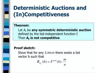
Deterministic Auctions and (In)Competitiveness. Proof sketch: Show that for any 1 mn there exists a bid vector b such that. Theorem: Let A f be any symmetric deterministic auction defined by the bid-independent function f. Then A f is not competitive.

E N D
Deterministic Auctions and (In)Competitiveness Proof sketch: Show that for any 1mn there exists a bid vector b such that Theorem: Let Af be any symmetric deterministic auction defined by the bid-independent function f. Then Af is not competitive.
Deterministic Auctions and (In)Competitiveness (Cont.) Proof sketch (cont.): • Fix m and n • Consider bid vectors whose bids are all n and 1 • Show that there is a bid vector b with k+1 ns such that Or else the solution is trivial. Thus:
Deterministic Auctions and (In)Competitiveness (Cont.) Proof sketch (cont.): Now: • If k+1<m we have:and: • Else - k+1m and:resulting with which proves the theorem
Competitive Auctions via Random Sampling • Randomly partition the bid vector b into two sets b’ and b’’ • Compute p’ based on b’ and p’’ based on b’’ • Assign the price p’ for b’’ and p’’ for b’ Two algorithms: • DSOT • SCS
Dual-Price Sampling Optimal Threshold Auction (DSOT) • Uses as the price setting mechanism • Constant competitive against F(2) • The bound is weak for the general case • Significantly better performance for some interesting special cases
DSOT – the Algorithm • Input: bid vector b • Output: Allocation vector x, price vector p • Randomly partition b into b’ and b’’ • Compute p’=opt(b’) and p’’ = opt(b’’) • Use p’ as a threshold for b’’ • Use p’’ as a threshold for b’
10 10 7 7 12 12 4 4 18 18 9 9 b’ = b’’ = 10 12 4 7 18 9 0 0 10 1 0 0 1 7 7 1 0 0 opt(b’) = 7 opt(b’’) = 10 x’ = x’’ = p’ = p’’ = DSOT - Example b =
DSOT – Performance Analysis • In the general case – DSOT is constant competitive against F (2); this bound is weak • For some interesting special cases DSOT’s performance is much better Example: If b is bounded-range bid vector (bi [1, h]) then
Sampling Cost-Sharing Auction (SCS) • Uses CostShareC for setting the price • At least 4-competitive against F(2) Definition (CostShareC): Given a cost C and bids b, find the largest k such that the highest k bid’s value C/k. Charge each C/k. • CostShareC is truthful • If (CF (b) then CostShareC has revenue of C; Otherwise it has no profit
SCS – the Algorithm • Input: bid vector b • Output: Allocation vector x, price vector p • Randomly partition b into b’ and b’’ • Compute F’=F(b’) and F’’=F(b’’) • Compute the auction results by running CostShareF’(b’’) and CostShareF’’(b’)
10 10 7 7 12 12 4 4 18 18 9 9 b’ = b’’ = 10 12 4 7 18 9 6 1 1 6 6 1 0 0 0 0 0 0 F(b’)=21 F(b’’)=20 x’ = x’’ = p’ = p’’ = SCS - Example b =
SCS – Performance Analysis Theorem: SCS is 4-competitive and this bound is tight Proof: • Assume F(b)=k·p then F’(b’)=k’·p’k’·p and F’’(b’’)=k’’·p’’k’’·p • If F’=F’’ then F’+F’’F(b) and we are done • Otherwise
SCS – Performance Analysis Proof (continue): • Expected value of min(k’,k’’): • Thus, the competitive ratio achieves its minimum of ¼ at k=2,3. as k increases, the ratio approaches ½
Bounded Supply • We may sell no more than k items • We wish to be competitive against F(m,k): Reduction to the unlimited supply case: • Reject any bid that is not among the k highest bids • Run the unlimited supply auction on the rest
Another look atCompetitive Analysis • Thus far we have compared performance to F, the optimal single-price auction • Is it “fair” to compare a dual-price auction to the optimal single-price auction? Theorem: for any monotone (truthful) randomized auction A, and for all bid vectors b, RA(b)=ipi satisfies E[R] F(b)
Monotonicity Definition (monotone auction): An auction is monotone if for any pair of bidders i and j with bi bj and for any t bi, we have Pr[(xi=1) (pit)] Pr[(xj=1) (pjt)] Intuition: • Since bi bj then b-i looks like a higher set of bids than b-j • We would expect a higher set of bids to yield a higher price
Hard-Coded Auctions For any bid vector b, there exists a truthful auction A that satisfies A(b)= T(b) • Example: • Consider the following auction A given by the bid-independent function f : Where’s the catch?
Monotonicity (Cont.) DSOT, SCS, Vickrey auctions are all monotone; so is F Thus F is the optimal monotone function Theorem: Let A be any monotone truthful randomized auction. For all bid vectors, the revenue of A satisfies E[R] F(b)
Summary • The notion of competitive auction was introduced • Justification for using F was given • It was shown that no deterministic auction may can be competitive • 2 novel randomized auctions for the unbounded supply scenario, DSOT and SCS were introduced • Reduction to the bounded supply was shown
Related Work • Cancelable auctions • Envy-free auctions • Almost truthful auctions • Online auctions