Download
1 / 24
240 likes | 364 Views
Climate Models, Projections of Future Sea Level Change, and Regional Variations. Jim Carton (UMD) & Laury Miller (NOAA) {thanks Ron Stouffer, Warren Lipscomb}. Outline. Global coupled models (IPCC approach) -- predict thermo., add ice-melt AR4: Bindoff et al., 2007; Meehl et al. 07

E N D
Climate Models, Projections of Future Sea Level Change, and Regional Variations Jim Carton (UMD) & Laury Miller (NOAA) {thanks Ron Stouffer, Warren Lipscomb}
Outline • Global coupled models (IPCC approach) -- predict thermo., add ice-melt • AR4: Bindoff et al., 2007; Meehl et al. 07 • AR5: GFDL, CCSM • Regional effects/downscaling • the AMOC: Yin et al. 09; Hu et al. 09; Kuhlbrodt et al. 09: max SLR 80cm • Downscaling to east coast (SAP4-1) • Semi-empirical approach • Ta -> SL Rahmstorf 07; Horton et al. 08; Grinsted et al. 09, etc. However: von Storch et al. 08 • Finger Printing -- model geoid adjustment to large ice-sheet melt
Third Assessment Report (TAR) (2001) A range sea level estimates was given: 0.09m to 0.88m by 2100 (Church 2001). (see: R. Pielke Jr. clarification) Fourth Assessment Report (AR4) (2007) • Included results from the Coupled Model Intercomparison Project Phase 3 (23 CGCMs) • Controls: 1860, 1990 • Emissions scenarios 2000-2100 • A1 (high emissions), • A1B (medium emissions), • B1 (low emissions)
Example: GFDL CM2.1 • Atmosphere/land 2°x2.5°x24lev • Radiative forcing: CO2, CH4, CFC11, 12, 22, 113, N2O, O3, natural (sea salt and dust) & anthropogenic aerosols (black carbon, organic carbon, and sulfate aerosols) • Runoff in drainage basins goes to ocean • Ocean MOM4, 1°x1° (1/3° near eq)x50lev • tripolar grid • true freshwater flux boundary condition • Sea ice: GFDL Sea Ice Simulator • one snow and two ice layers • No: continental ice (but some hosing expts.), tides, gravitational effects
AR4 SLR Ensemble Projection “Thermal expansion is projected to contribute more than half of the average rise, but land ice will lose mass increasingly rapidly as the century progresses. An important uncertainty relates to whether discharge of ice from the ice sheets will continue to increase as a consequence of accelerated ice flow, as has been observed in recent years. This would add to the amount of sea level rise, but quantitative projections of how much it would add cannot be made with confidence”. (Bindoff et al., 2007) 20-50cm by 2100 (4mm/yr by 2190) AR4 neglected “full effects of changes in ice sheet flow” but did include current rates of Greenland and AA melt. Suggest +10—20cm TAR Fig 1 from Chapter 5: SLR under A1B
Post-AR4 • Problems with Obs heat content record have been addressed • Mass contributions from melting land ice larger than expected and apparently growing • Global emissions have continued to increase in excess of A1F1 Models are at the low range of obs tide gaugesaltimetry Model estimates (updated from Rahmstorf, et al., Sci., 2007)
GFDL for AR5 *public release: 2013
NCAR’s CCSM for AR5 websrv.cs.umt.edu/isis/index.php/Coupling_the_Cryosphere_to_other_Earth_systems%2C_part_II
CCSM: exploring the impact of continental ice melt (activity of the Land Ice working group) With CCSM3 its been found that a melting rate exceeding 0.05 Sv would weaken the MOC by 9-24% by the end of the 21st century. CMWG has proposed 2009 experiments with 200yr T42 CCSM3 simulations: 1. West Antarctic ice sheet melting via a constant melting rate of 0.004 Sv (Antartica 2002-2006: 0.0033 Sv; 2006-2009: 246 Gt/year = 0.0078 Sv = 246Gt/yr) 2. Same as 1, but with increase 1% per year (0.04Sv at yr100). 3. Same as 1, but with increase 3% per year (1.34Sv at yr100) 4. Same as 1, but with increase 7% per year (2.91Sv at yr100) 5. Same as 3, but with global runoff increase of 3% per year 6. Same as 5, but adding Greenland melting with 3% increase (2002-2006: 0.0043 Sv; 2007-2009: 0.0091 Sv) Ice modeling initiatives: EU: Ice2sea, SeaRISE
AR4 Changes in the AMOC A1b emissions GFDL CM2.1 All emission scenarios Meehl et al. 2007
AR4 10-model Mean SLR 2091-2100 wrt to 1981-2000, ten models, A1B medium emission scenario Over next 100 years, dynamic SLR very uneven (Yin, et al., 2009)
Impact of excess meltwater in Potsdam’s Climber-3α SLA1FI_090 - SLA1FI_000 in 2150{A1FI_090 includes 0.09 Sv/K meltwater} Up to 80 cm Kuhlbrodt et al. 2009
GFDL CM2.1 Model Simulation vs. Observed Dyn SSH Observed Dynamic SSH (1992-2002) Simulated Dynamic SSH (1992-2002) Simulation produces realistic Gulf Stream, Subtropical & Subpolar Gyres (Yin, et al., 2009)
CM2.1 A1B Scenario: Steric vs. Mass Contributions to SSH Steric SSH Anomaly A1B Scenario (2091-2100 wrt 1981-2000) Mass SSH Anomaly A1B Scenario (2091-2100 wrt 1981-2000) Sharp steric SSH gradient across shelf break can’t be balanced by geostrophy, consequently mass loading along NE coastline. (Mass redistribution calculated on basis of bottom pressure change) Decrease in AMOC decrease in production of NADW increase in steric SLR along path of DWBC (Yin, et al., 2009)
Eq. 2 Eq. 1 Predicting SLR from Ta • Rate of SLR proportional to magnitude of warming global mean surface temperature above pre-industrial Age. SL adjusts exponentially to temperature with a timescale of several hundred years as the heat gradually penetrates the deep ocean. • Uses LSQR estimation of “a” from observations, combined with temperature projections from TAR (R07) and AR4(H08,G09) to estimate SLR • Drawbacks: Estimation of coefficient “a” problematic due to inadequate observations; method doesn’t allow for non-linear ice melt processes Rahmstorf 2007, extended by Horton et al. 2008, Grinsted et al. 2009
Estimating Coefficient “a” • Correlation of T and dH/dt for period 1881-2001 • Both T and H curves smoothed by computing non-linear trends over 15 years • dH/dt estimated by taking derivative of H curve • Data binned in 5 yr avgs Method relies on heavy smoothing, resulting in small number of degrees of freedom. (Rahmstorf, 2007)
dH/dt from tide gauges dH/dt from dT (eq. 1) dH from tide gauges dH from integral of (eq. 1) SLR hindcast based on surface temperature observations (Rahmstorf, 2007)
von Storch, et al. (2008) counters: Based on ECHO-G simulation (which admittedly doesn’t include all physical processes), neither dT or dT/dt are reliable predictors of dH/dt. Although some agreement on centennial scales, there are intervals of large errors and even inverse relationship. In general, the semi-empirical approach is problematic. It relies on the statistics of a short, heavily smoothed observational record, that is highly autocorrelated, and has strong trends.
Item #3: What type of observations and research activities should be encouraged in order to improve sea level projections for the 21st century? • Need to get the obs and modeling communities to work together • Must monitor ice (continental and sea)! We need to know the range of possible acceleration • Must monitor salinity, particularly at high latitude • Need to improve Arctic Ocean processes
References • Horton, R., C. Herweijer, C. Rosenzweig, J. Liu, V. Gornitz and A.C. Ruane (2008). Sea level rise projections for Current generation CGCMs based on the semi-empirical method. Geophysical Research Letters, 35: L02725, doi:10.1029/2007GL032468. • Hu, A., G.A. Meehl, W. Han, and J. Yin, 2009: Transient response of the MOC and climate to potential melting of the Greenland Ice Sheet in the 21st century, Geophys. Res. Letts., 36, L10707, doi:10.1029/2009GL037998. • Kuhlbrodt, T., et al., 2009: An Integrated Assessment of changes in the thermohaline circulation, Climatic Change, 96, 489–537, DOI 10.1007/s10584-009-9561-y • Meehl et al, 2005: How Much More Global Warming and Sea Level Rise? Science, 307,1769 – 1772. • Rahmstorf, S., 2007: A Semi-Empirical Approach to Projecting Future Sea-Level Rise, Science, 315, 368 – 370. also: Response to comments on "A semi-empirical approach to projecting future sea-level rise“, Science, 317, 5846. • Sen Gupta A, A. Santoso A., AS Taschetto, CC Ummenhofer, J. Trevena, MH England, 2009: Projected Changes to the Southern Hemisphere Ocean and Sea Ice in the IPCC AR4 Climate Models, J. Clim., 22, 3047-3078. • Tamsiea, M. E., J.X. Mitrovica, J.L. Davis, and G.A. Milne, 2003: II: SOLID EARTH PHYSICS: Long Wavelength Sea Level and Solid Surface Perturbations Driven by Polar Ice Mass Variations: Fingerprinting Greenland and Antarctic Ice Sheet Flux, Space Science Reviews, 108, 1572-, 10.1023/A:1026178014950 • Velicogna, I. (2009), Increasing rates of ice mass loss from the Greenland and Antarctic ice sheets revealed by GRACE, Geophys. Res. Letts., 36, L19503, doi:10.1029/2009GL040222 • von Storch H, E. Zorita, JF Gonzalez-Rouco, 2008: Relationship between global mean sea-level and global mean temperature in a climate simulation of the past millennium, Ocean Dynam., 58, 227-236. • Yin, J., M.E. Schlesinger, and R.J. Stouffer, 2009: Model projections of rapid sea-level rise on the northeast coast of the United States, Nature Geosci., DOI: 10.1038/NGEO462