Extrapolation of magnetic fields

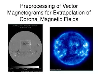
1. Extrapolation of magnetic fields Thomas Wiegelmann • Why study coronal magnetic fields? • How to obtain the coronal magnetic field vector? • Linear and non-linear models. • Computational implementation and tests. • Recent problems and possible solutions. • Evolution of coronal fields and flare prediction. • Outlook: Coronal plasma and dynamics.

2. It is important to investigate the coronal magnetic field Coronal mass ejections and flares are assumed to occur due to instabilities in the coronal magnetic field configuration.

3. Coronal magnetic Fields: Origin of Space weather Question: Origin of coronal eruptions

4. Solar magnetic field measured routinely only in photosphere Aim: Extrapolate measured photospheric magnetic field into the corona under model assumptions.

5. How to model the stationary Corona? Force-free Fields Low plasma Beta in corona Lorentz force pressure gradient gravity Neglect plasma pressure+gravity

6. Force-Free Fields Equivalent • Potential Fields (no currents) • Linear force-free fields (currents globally proportional to B-field) Relation between currents and magnetic field. Force-free functions is constant along field lines, but varies between field lines. => nonlinear force-free fields Further simplifications

7. Easy to computeRequire only LOS-Magnetograms Here: global constant linear force-free parameter

8. Potential Field Model EUV-emission Simple potential field models provide already a reasonable estimate regarding the global magnetic field structure. Mainly closed loops in active regions and open field lines in coronal holes.

9. Active Regions EIT-image and projections of magnetic field lines for a potential field (α=0) . (bad agreement) Linear force-free field with α=+0.01 [Mm-1] (bad agreement) We use a linear force-free model with MDI-data and have the freedom to choose an appropriate value for the force-free parameter α.

10. Linear force-free field with α=-0.01 [Mm-1] (good agreement) 3D-magnetic field lines, linear force-free α=-0.01 [Mm-1]

11. NonLinear Force-Free Fields Equivalent • Compute initial a potential field (Requires only Bn on bottom boundary) • Iterate for NLFFF-field, Boundary conditions:- Bn and Jn for positive or negative polarityon boundary (Grad-Rubin)- Magnetic field vector Bx By Bz on boundary (Magnetofrictional,Optimization)

12. Grad-Rubin methodSakurai 1981, Amari et al. 1997,2006, Wheatland 2004,06,07

13. Magnetofrictional Chodura & Schlueter 1981, Valori et al. 2005 Optimization Wheatland et al. 2000, Wiegelmann 2004,2007

14. Test: Model Active Region (van Ballegooijen et al. 2007, Aad’s model) Model contains the (not force-free) photospheric magnetic field vector and an almost force-free chromosphere and corona.

15. Grad-Rubin MHD-relaxation Optimization Comparison paper, Metcalf et al., Sol. Phys. 2008. -Good agreement for extrapolations from chromosphere. -Poor results for using photospheric data directly. -Improvement with preprocessed photospheric data.

16. Force-Free B-Field Measurements, non-force-free

17. If these relations are NOT fulfilled on the boundary, then the photospheric data are inconsistent with the force-free assumption. NO Force-Free-Field. Consistency criteria for vectormagnetograms (Aly 1989)

18. No net force No net torque Photosphere Smoothness Preprocessed boundary data

19. Chromospheric H-alpha preprocessing • H-alpha fibrils outline magnetic field lines. • With image-recognition techniques we gettangent to the chromospheric magnetic fieldvector (Hx, Hy). • Idea: include a term in the preprocessing tominimize angle of preprocessed magnetic field (Bx,By) with (Hx,Hy).

20. Preprocessing can be improved by including chromospheric observations. (Wiegelmann, Thalmann, Schrijver, DeRosa, Metcalf, Sol. Phys. 2008) Preprocessing of vector magnetograms(Wiegelmann, Inhester, Sakurai, Sol. Phys. 2006) • Use photospheric field vector as input. • Preprocessing removes non-magneticforces from the boundary data. • Boundary is not in the photosphere (which is NOT force-free). • The preprocessed boundary dataare chromospheric like.

21. We test preprocessing with Aad’s model Prepro- cessing

22. Results: Comparison with Aad‘s Model

23. H-AlphaImage Vector magnetogram Optional Preprocessing tool Chromospheric Magnetic Field Nonlinear Force-free code Coronal Magnetic Field

24. Comparison of observed magnetic loops and extrapolations from photospheric measurements Nonlinear force-free Models are superior. Potential field reconstruction Linear force-free reconstruction Non-linear force-free reconstruction Measured loops in a newly developed AR (Solanki, Lagg, Woch, Krupp, Collados, Nature 2003)

25. Stereoscopy vs. coronal field extrapolation Hinode FOV From DeRosa et al. 2009: Blue lines are stereoscopic reconstructed loops (Aschwanden et al 2008), Red lines nonlinear force-free extrapolated field lines from Hinode/SOT with MDI-skirt.

26. Stereoscopy vs. coronal field extrapolation • Vector magnetogram data (here: Hinode/SOT) areessential for nonlinear force-free field modeling. • Unfortunately Hinode-FOV covered only a smallfraction (about 10%) of area spanned by loopsreconstructed from STEREO-SECCHI images. • Quantitative comparison was unsatisfactory,NLFFF-models not better as potential fields here. • In other studies NLFFF-methods have shown to besuperior to potential and linear force-freeextrapolations. (Comparison with coronal images from one viewpoint, NLFFF-models from ground based data)

27. Results of NLFFF-workshop 2008 • When presented with complete and consistent boundary conditions, NLFFF algorithms succeed in modeling test fields. • For a well-observed dataset (a Hinode/SOT-SP vector-magnetogram embedded in MDI data) the NLFFF algorithms did not yield consistent solutions. From this study we conclude that one should not rely on a model-field geometry or energy estimates unless they match coronal observations. • Successful application to real solar data likely requires at least: • large model volumes at high resolution that accommodate most of the connectivity within a region and to its surroundings; • accommodation of measurement uncertainties (in particular in the transverse field component) in the lower boundary condition; • 'preprocessing’ of the lower-boundary vector field that approximates the physics of the photosphere-to-chromosphere interface as it transforms the observed, forced, photospheric field to a realistic approximation of the high-chromospheric, near-force free field. • See: Schrijver et al. 2006 (Spy 235, 161), 2008 (ApJ 675, 1637), Metcalf et al. 2008 (SPh 247, 269), DeRosa et al. (2009, ApJ 696, 1780).

28. Temporal Evolution of Active Regions Use time series of ground based vector magnetograms with sufficient large FOV (Solar Flare Telescope, SOLIS).

29. Flaring AR-10540 (Thalmann & Wiegelmann A&A 2008) M6.1 Flare Magnetic energy buildsup and is releases during flare Active Region-10960 Solar X-ray flux. Vertical blue lines: vector magnetograms available Magnetic field extrapolations from Solar Flare telescope Extrapolated from SOLIS vector magnetograph

30. Comparison of two Active Regions

31. Conclusions • Potential and linear force-free fields are popular due to their mathematic simplicity and because only LOS-magnetogramsare needed as input. • Non-linear force-free fields model coronal magnetic fields more accurately [energy, helicity, topology etc.]. • Nonlinear models are mathematical very challenging and require high quality photospheric vector magnetograms as input. • We still need to understand the physics of the interface-region between high beta photosphere, where the magnetic field vectoris measured, and the force-free corona. • Coronal magnetic field models should be compared andvalidated by coronal observations.

32. 3D EUV loops 3D field lines Scaling laws Stereoscopy Tomography Plasma along magnetic loops Artificial images 3D Force-free magnetic field LOS-integration Self-consistent equilibrium Time-dependent MHD-simulations Vector magnetogram Where to go in corona modeling? STEREO images Force-free code consistent? compare MHS code