Dynamics and Steady States of Two Chemostats in Series

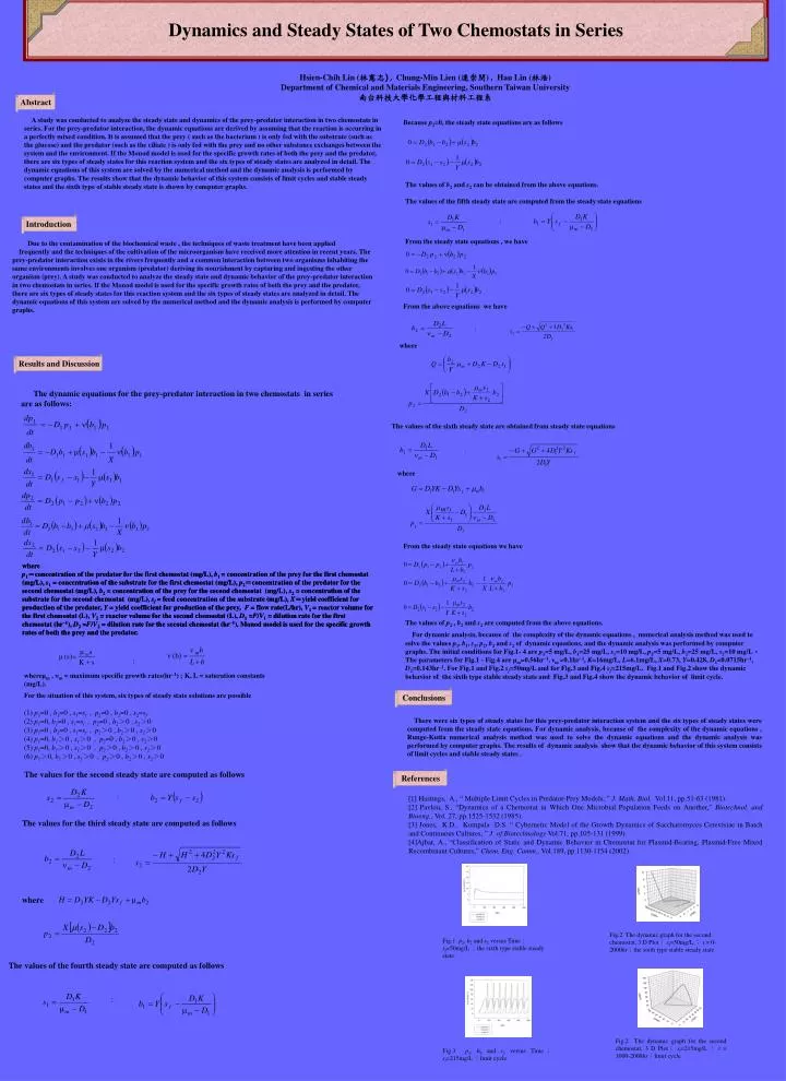
1. Dynamics and Steady States of Two Chemostats in Series Hsien-Chih Lin (林憲志),Chung-Min Lien (連崇閔) , Hau Lin (林浩) Department of Chemical and Materials Engineering, Southern Taiwan University 南台科技大學化學工程與材料工程系 Abstract A study was conducted to analyze the steady state and dynamics of the prey-predator interaction in two chemostats in series. For the prey-predator interaction, the dynamic equations are derived by assuming that the reaction is occurring in a perfectly mixed condition. It is assumed that the prey ( such as the bacterium ) is only fed with the substrate (such as the glucose) and the predator (such as the ciliate ) is only fed with the prey and no other substance exchanges between the system and the environment. If the Monod model is used for the specific growth rates of both the prey and the predator, there are six types of steady states for this reaction system and the six types of steady states are analyzed in detail. The dynamic equations of this system are solved by the numerical method and the dynamic analysis is performed by computer graphs. The results show that the dynamic behavior of this system consists of limit cycles and stable steady states and the sixth type of stable steady state is shown by computer graphs. Because p2=0, the steady state equations are as follows ； The values of b2 and s2 can be obtained from the above equations. The values of the fifth steady state are computed from the steady state equations Introduction ； From the steady state equations , we have Due to the contamination of the biochemical waste , the techniques of waste treatment have been applied frequently and the techniques of the cultivation of the microorganism have received more attention in recent years. The prey-predator interaction exists in the rivers frequently and a common interaction between two organisms inhabiting the same environments involves one organism (predator) deriving its nourishment by capturing and ingesting the other organism (prey). A study was conducted to analyze the steady state and dynamic behavior of the prey-predator interaction in two chemostats in series. If the Monod model is used for the specific growth rates of both the prey and the predator, there are six types of steady states for this reaction system and the six types of steady states are analyzed in detail. The dynamic equations of this system are solved by the numerical method and the dynamic analysis is performed by computer graphs. From the above equations we have ； where Results and Discussion The dynamic equations for the prey-predator interaction in two chemostats in series are as follows: The values of the sixth steady state are obtained from steady state equations ； where From the steady state equations wehave where p1＝concentration of the predator for the first chemostat (mg/L), b1= concentration of the prey for the first chemostat (mg/L), s1= concentration of the substrate for the first chemostat (mg/L), p2＝concentration of the predator for the second chemostat (mg/L), b2= concentration of the prey for the second chemostat (mg/L), s2= concentration of the substrate for the second chemostat (mg/L), sf = feed concentration of the substrate (mg/L), X＝yield coefficient for production of the predator, Y = yield coefficient for production of the prey, F = flow rate(L/hr), V1= reactor volume for the first chemostat (L), V2= reactor volume for the second chemostat (L), D1=F/V1= dilution rate for the first chemostat (hr–1), D2=F/V2= dilution rate for thesecond chemostat (hr–1).Monod model is used for the specific growth rates of both the prey and the predator. where p1＝concentration of the predator for the first chemostat (mg/L), b1= concentration of the prey for the first chemostat (mg/L), s1= concentration of the substrate for the first chemostat (mg/L), p2＝concentration of the predator for the second chemostat (mg/L), b2= concentration of the prey for the second chemostat (mg/L), s2= concentration of the substrate for the second chemostat (mg/L), sf = feed concentration of the substrate (mg/L), X＝yield coefficient for production of the predator, Y = yield coefficient for production of the prey, F = flow rate(L/hr), V1= reactor volume for the first chemostat (L), V2= reactor volume for the second chemostat (L), D1=F/V1= dilution rate for the first chemostat (hr–1), D2=F/V2= dilution rate for thesecond chemostat (hr–1).Monod model is used for the specific growth rates of both the prey and the predator. The values of p2 , b2 and s2 are computed from the above equations. For dynamic analysis, because of the complexity of the dynamic equations , numerical analysis method was used to solve the values p1, b1, s1, p2, b2 and s2 of dynamic equations, and the dynamic analysis was performed by computer graphs. The initial conditions for Fig.1- 4 are p1=5 mg/L, b1=25 mg/L, s1=10 mg/L, p2=5 mg/L, b2=25 mg/L, s2=10 mg/L。The parameters for Fig.1 - Fig.4 are μm=0.56hr–1, νm =0.1hr–1, K=16mg/L, L=6.1mg/L, X=0.73, Y=0.428, D1=0.0715hr–1, D2=0.143hr–1. For Fig.1 and Fig.2 sf=50mg/L and for Fig.3 and Fig.4 sf=215mg/L. Fig.1 and Fig.2 show the dynamic behavior of the sixth type stable steady state and Fig.3 and Fig.4 show the dynamic behavior of limit cycle. ； whereμm , m = maximum specific growth rates(hr–1) ; K, L = saturation constants (mg/L). Conclusions For the situation of this system, six types of steady state solutions are possible (1) p1=0 , b1=0 , s1=sf , p2=0 , b2=0 , s2=sf (2) p1=0, b1=0 , s1=sf , p2=0 , b2＞0 , s2＞0 (3) p1=0 , b1=0 , s1=sf , p2＞0 , b2＞0 , s2＞0 (4) p1=0, b1＞0 , s1＞0 , p2=0 , b2＞0 , s2＞0 (5) p1=0, b1＞0 , s1＞0 , p2＞0 , b2＞0 , s2＞0 (6) p1＞0, b1＞0 , s1＞0 , p2＞0 , b2＞0 , s2＞0 The values for the second steady state are computed as follows There were six types of steady states for this prey-predator interaction system and the six types of steady states were computed from the steady state equations. For dynamic analysis, because of the complexity of the dynamic equations , Runge-Kutta numerical analysis method was used to solve the dynamic equations and the dynamic analysis was performed by computer graphs. The results of dynamic analysis show that the dynamic behavior of this system consists of limit cycles and stable steady states . References [1] Hastings, A., “ Multiple Limit Cycles in Predator-Prey Models, ” J.Math. Biol. Vol.11, pp.51-63 (1981). [2] Pavlou, S., “Dynamics of a Chemostat in Which One Microbial Population Feeds on Another,” Biotechnol. and Bioeng., Vol. 27, pp.1525-1532 (1985). [3]Jones, K.D., Kompala D.S. “Cybernetic Model of the Growth Dynamics of Saccharomyces Cerevisiae in Batch and Continuous Cultures, ” J. of Biotechnology Vol.71, pp.105-131 (1999). [4]Ajbar, A., “Classification of Static and Dynamic Behavior in Chemostat for Plasmid-Bearing, Plasmid-Free Mixed Recombinant Cultures,” Chem. Eng. Comm., Vol.189, pp.1130-1154 (2002). ； The values for the third steady state are computed as follows ； where Fig.2 The dynamic graph for the second chemostat, 3 D Plot； sf=50mg/L； t = 0-2000hr；the sixth type stable steady state Fig.1 p2, b2 and s2 versus Time； sf=50mg/L ；the sixth type stable steady state The values of the fourth steady state are computed as follows ； Fig.2 The dynamic graph for the second chemostat, 3 D Plot； sf=215mg/L； t = 1000-2000hr；limit cycle Fig.3 p2, b2 and s2 versus Time； sf=215mg/L；limit cycle