Download
1 / 17
170 likes | 274 Views
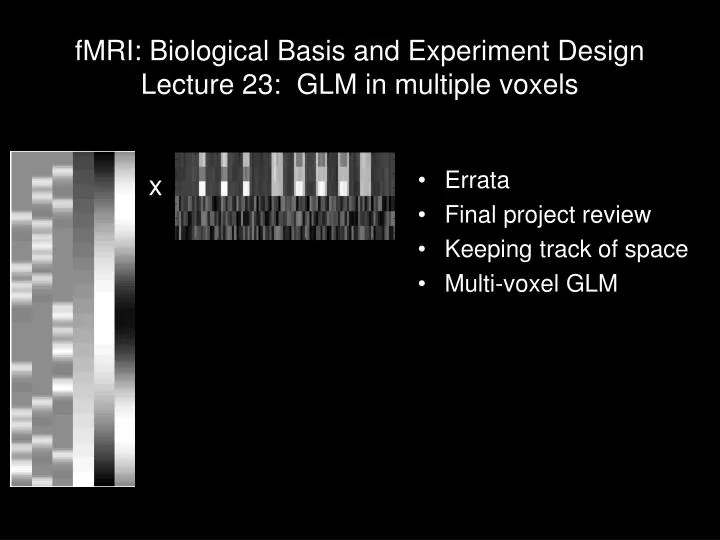
fMRI: Biological Basis and Experiment Design Lecture 23: GLM in multiple voxels. Errata Final project review Keeping track of space Multi-voxel GLM. Before. x. After. Erratum: ICE9. % Repeat the "experiment" a few times

E N D
fMRI: Biological Basis and Experiment DesignLecture 23: GLM in multiple voxels • Errata • Final project review • Keeping track of space • Multi-voxel GLM Before x After
Erratum: ICE9 % Repeat the "experiment" a few times %%%!!! Wrong way ... shouldn't run the same design again and again - then %%%the experimental conditions aren't nearly as randomized as they could %%%be! nScans = 10; clear data for n = 1:nScans data(n,:) = caoSimulateData(neural,TR,BOLDamp,SNR,1); end % "Analyze" data ... % %Check out code that does TTA ... TTAlength = 20; [TTA TTAsem count] = caoComputeTTA(design,data,TTAlength); TTA_minus_baseline = TTA - repmat(TTA(:,1),[1 size(TTA,2)]); subplot(2,1,1) errorbar(repmat((0:(TTAlength-1))',[1 size(TTA,2)]),TTA,TTAsem); title(['nScans = ' num2str(nScans)]); axis tight subplot(2,1,2) errorbar(repmat((0:(TTAlength-1))',[1 size(TTA,2)]),TTA_minus_baseline,TTAsem); title(['nScans = ' num2str(nScans)]); axis tight legend(num2str(count))
Erratum: ICE9 % Repeat the "experiment" a few times %% Right way - new trial order each repetition nScans = 10; fixedLength = 500; design = zeros(nScans,fixedLength); neural = zeros(nScans,fixedLength); data = zeros(nScans,fixedLength); for n = 1:nScans %% For this, I'd built in a flag that would make the design vector the %% same length each time (adding 0's at end) to deal with the fact that %% randomized ISI's yield unpredictable scan lengths design(n,:) = caoMakeER(waitUpFront,nStimTypes,ISIrange,nStim,500); for nt = 1:length(design) if design(n,nt) % if there's a stimulus neural(n,nt) = relResp(design(n,nt)); % pick the appropriate response end end data(n,:) = caoSimulateData(neural(n,:),TR,BOLDamp,SNR,1); end
Basic assignment, final project(all projects need these components) • Abstract (250 words) • Background - experiment design and neuroscience question motivating the experiment (1 page, 1 - 3 references) • Methods (2 – 4 pages) • MR Methods section (resolution, TR, TE, protocol) • Prediction of neural activity • Prediction of BOLD response (noiseless model) • Simulated data (BOLD + noise - physiological and/or thermal) • ROI selection • GLM • Results (1 – 3 pages) • Paragraph describing simulation output + 1 figure • Paragraph describing GLM results + 1 figure • Discussion (1 - 2 pages) • 3 things that might not be as expected if you ran the experiment
Building blocks, final project(weekly assignments, 2nd half of semester) • Abstract (250 words) • Background - experiment design and neuroscience question motivating the experiment (1 page, 1 - 3 references) • Methods (2 – 4 pages) • MR Methods section (resolution, TR, TE, protocol) – WA 8 • Prediction of neural activity – WA7 • Prediction of BOLD response (noiseless model) – WA7 • Simulated data (BOLD + noise - physiological and/or thermal) – WA8 • ROI selection • GLM – WA10 & WA11 • Results (1 – 3 pages) • Paragraph describing simulation output + 1 figure – WA8 • Paragraph describing GLM results + 1 figure – WA10 & WA11 • Discussion (1 - 2 pages) • 3 things that might not be as expected if you ran the experiment
Groups Denkinger Han, Honwanishkul, Roher Haut, Johnson Kruse, White Kwon Liu, Schmidt Seo, Vizueta Theodorou Thompson Times May 2 9:45 – 10:05 Kwon 10:05 – 10:25 Theodorou 10:25 – 10:45 Denkinger 10:45 – 11:15 Big group HHR May 4 9:45 – 10:05 Thompson 10:05 – 10:25 Big group 10:25 – 10:45 Seo, Vizueta 10:45 – 11:15 Haut, Johnson Presentation schedule
Linear model for BOLD in a single voxel Ax = y Design matrix, [m x n] - m time-points - n stimulus types Data [m x 1] - response through time Responses [n x 1] - for each stimulus, a scalar (single number) representing how well that voxel responds to that stimulus y1 y2 y3 ym x1 x2 x3 x4 A1,1 A2,1 A3,1 A4,1 A1,2 A2,2 A3,2 A4,2 A1,3 A2,3 A3,3 A4,3 A1,m A2,m A3,m A4,m A = x = y = ... ... ... ... ...
Linear model for BOLD in multiple voxels Ax = y Design matrix, [m x n] - m time-points - n stimulus types Data [m x p] - response through time Responses [n x p] - for each stimulus, a scalar (single number) representing how well that voxel responds to that stimulus y1,1 y2,1 y3,1 ym,1 y1,2 y2,2 y3,2 ym,2 y1,p y2,p y3,p ym,p x1,1 x2,1 x3,1 x4,1 x1,2 x2,2 x3,2 x4,2 x1,p x2,p x3,p x4,p A1,1 A2,1 A3,1 A4,1 A1,2 A2,2 A3,2 A4,2 A1,3 A2,3 A3,3 A4,3 A1,m A2,m A3,m A4,m ... ... ... ... A = x = y = ... ... ... ... ... ... ... ... ... ... ...
Keeping track of voxels 1D vector X & Y (& Z) coords 2D (or 3D) array of data = +
Fake experiment – distributed neural activity Brain (3 types of responses) 3 types of stimuli; 3 types of "neuron" (voxel?)
Fake experiment – simulated data Brain (3 types of responses) voxels (Baseline trends, noise dominate visualization)
Design Matrix - Stimulus 1 - Stimulus 2 - Stimulus 3 - Linear drift - Half-cycle cos drift - 1.5 cycle cos drift
Design Matrix + (sim.) data voxels voxels ? X = time
(An aside on rows and columns) • Why do [nTpts nVoxels] instead of [nVoxels nTpts]? • Typical experiment • 6 scans, 200 tpts per scan --> nTpts = 1200 • 1 brain, 64 x 64 x 30 voxels --> nVoxels = 122,880 • Size of A • [nTpts nVoxels]: [122,880 1200] • [nVoxels nTpts]: [1200 122,880] • Size of ATA • [nTpts nVoxels]: [1200 1200] • [nVoxels nTpts]: [122,880 122,880] !
Estimate of voxel responses voxels xest = x + = (ATA)-1AT (y + ) X = time voxels
Estimate of voxel responses Estimated Response to Stim1 Response to Stim2 Response to Stim3 Input