Download
1 / 48
490 likes | 664 Views
MST Algorithms. Kruskal’s Algorithm Disjoint Sets Prim’s Algorithms. Implementing Kruskal’s Algorithm. Initially, the MST has |V| vertices and 0 edges (A = ) While A is not an MST Find the cheapest edge not yet considered If you add it to A, would you induce a cycle?

E N D
MST Algorithms Kruskal’s Algorithm Disjoint Sets Prim’s Algorithms
Implementing Kruskal’s Algorithm • Initially, the MST has |V| vertices and 0 edges (A = ) • While A is not an MST • Find the cheapest edge not yet considered • If you add it to A, would you induce a cycle? • If not, add it to A
Disjoint Sets • Initially each vertex is a connected component • Represent each connected component as a set. The sets are disjoint. • When considering an edge, determine if the two endpoints are in the same connected component (disjoint set).
15 f a 8 6 13 10 d b 11 g 13 7 14 e c 9
d f 6 b c 7 a d 8 c e 9 b e 10 d e 11 f g 13 a b 13 e g 14 a f 15 f a d b g e c
b c 7 a d 8 c e 9 b e 10 d e 11 f g 13 a b 13 e g 14 a f 15 f a d b g e c
a d 8 c e 9 b e 10 d e 11 f g 13 a b 13 e g 14 a f 15 f a d b g e c
c e 9 b e 10 d e 11 f g 13 a b 13 e g 14 a f 15 f a d b g e c
b e 10 d e 11 f g 13 a b 13 e g 14 a f 15 f a d b g e c
d e 11 f g 13 a b 13 e g 14 a f 15 f a d b g e c
f g 13 a b 13 e g 14 a f 15 f a d b g e c
a b 13 e g 14 a f 15 f a d b g e c
Chapter 22 Data Structures for Disjoint Sets • Problem: Maintain a collection of disjoint dynamic sets S = {S1, S2,..., Sn} • each set is identified by a representative • a representative is some member of the set • often does not matter which element is the representative • if we ask for the representative two times in succession without modifying the set, we should get the same answer • each element represented by an object
Operations • MAKE-SET(x) • create a new set whose only member is x • the representative will also be x • x cannot already be in a set (disjoint) • UNION(x,y) • create a new set that is the union of the set containing x and set containing y • destroy old set (maintain disjoint sets) • FIND-SET(x) • return a pointer to the representative of the set containing x
ANALYSIS OF SEQUENCE OF OPERATIONS • Amortized analysis • Analysis in terms of two parameters • n number of MAKE-SET operations • m total number of operations • How many sets after n-1 unions? • The constraint m n holds. Why?
Linked List Representation • Each set represented as a linked list • Each node of a list contains • the object • a pointer to the next item in the list • a pointer back to the representative for the set
x={c, h, e, b} c h e b f g d y={f, g, d}
c h e b f g d x y = {c, h, e, b, f, g, d} Union of the Two Sets x and y
Node Next Rep d f 6 b c 7 a d 8 c e 9 b e 10 d e 11 f g 13 a b 13 e g 14 a f 15 a nil a b nil b c nil c d nil d e nil e f nil f g nil g
Node Next Rep b c 7 a d 8 c e 9 b e 10 d e 11 f g 13 a b 13 e g 14 a f 15 a nil a b nil b c nil c d f f e nil e f nil f g nil g
Node Next Rep a d 8 c e 9 b e 10 d e 11 f g 13 a b 13 e g 14 a f 15 a nil a b c b c nil b d f d e nil e f nil d g nil g
Node Next Rep c e 9 b e 10 d e 11 f g 13 a b 13 e g 14 a f 15 a d a b c b c nil b d f a e nil e f nil a g nil g
Node Next Rep b e 10 d e 11 f g 13 a b 13 e g 14 a f 15 a d a b c b c e b d f a e nil b f nil a g nil g
Node Next Rep d e 11 f g 13 a b 13 e g 14 a f 15 a d a b c b c e b d f a e nil b f nil a g nil g
Node Next Rep f g 13 a b 13 e g 14 a f 15 a d a b c b c e b d f a e nil b f e b g nil g
Time Complexity of Operations • MAKE-SET(x) • O(?) • FIND-SET(x) • O(?) • UNION(x,y) • append x to y. • time is linear in length of x • O(?)
Time Complexity of a Series of Operations • Suppose we have m operations • All m are UNION • Max size of a set is n • So complexity in worst case would be O(m(n-1))= O(m2) • Can we do better with amortized analysis?
Operation Number of objects updated MAKE-SET(x1) 1 MAKE-SET(x2) 1 . . . MAKE-SET(xn) 1 UNION(x1, x2 ) 1 UNION(x2, x3 ) 2 UNION(x3, x4 ) 3 . . UNION(xq-1, xq ) q-1 where q = m - n
Analysis of Complexity • n = m/2 • q = m - n = m/2- 1 • Execute sequence of m = q + n operations • MAKE-SET O(n) • Total updates by UNION • Total time (n + q2) • Since n = m) and q = m) • Total time is (m2) • Amortized cost per operation is (m) • No improvement!
Weighted Union Heuristic • Obvious thing to try – always append the shortest list to the end of the longest • Question: Will this give us any asymptotic improvement in performance? • In order to implement, just keep the number of items in the set with the representative.
Theorem 22.1 • Using the linked-list representation of disjoint sets and the weighted-union heuristic, a sequence of m MAKE-SET, UNION, and FIND-SET operations, n of which are MAKE-SET operations, takes O(m + n lg n) time.
Proof • For each object, compute an upper bound on the number of times its representative pointer was updated. • Remember that x will be in the smaller set when its representative is updated • first update result has at least 2 elements • second update result has at least 4 elements • lg k update result has at least k elements (k<=n) • Since there are at most n elements, there have been at most lg n updates of any one element • Total time for updating is O(n lg n) • Total time for m operations is O(m + n lg n)
Another Improvement • Use trees to represent each set instead of linked lists • Each member points to its parent only. • Root points to itself • Straightforward implementation is no faster than linked list • Two heuristics can make it very fast
c f f e h d c d b e h g g b UNION(e,g)
Operations • MAKE-SET creates a tree with one node • FIND-SET chases pointers back to the parent • nodes on this path constitute the “find path” • UNION causes the root of one tree to point to the root of the other
Analysis • A series of n UNION operations could create a tree that is a linear chain of n nodes. • A FIND-SET operation could then require O(n) • Sequence of m operations is still O(m2)
Heuristics to Improve Running Time • Union by rank • make the root of the tree with fewer nodes point to the root of the tree with more nodes • each node will have a value called a rank that approximates the logarithm of the subtree size (is also an upper bound on the height of the node) • In union by rank, the root with smaller rank is made to point to the root with larger rank during a UNION operation.
Path Compression • Use during FIND-SET operations to make each node on the find path point directly to the root. • Path compression does not change ranks.
e d e c d c b b a a
Implementation • With each node x, maintain an integer rank[x] (upper bound of height) • rank[x] is 0 for a new subtree made with MAKE-SET • FIND-SET leaves rank unchanged • UNION makes the root of higher rank the root of the new tree • p[x] is the parent of x
MAKE-SET(x) 1 p[x] <- x 2 rank[x] <- 0 UNION(x,y) 1 LINK(FIND-SET(x), FIND-SET(y)) LINK(x,y) 1 if rank[x] > rank[y] 2 then p[y] <- x 3 else p[x] <-y 4 if rank[x] = rank[y] 5 then rank[y] = rank[y] + 1
FIND-SET(x) 1 if x <> p[x] 2 then p[x] <- FIND-SET(p(x)) 3 return p[x]
Disjoint Sets as a Trees • Heuristics for improving performance • Union by rank • Path compression • Running time using both heuristics • O(m(m,n)) • (m,n) is inverse of Ackermann’s function • (m,n) is essentially constant for almost all conceivable applications of a disjoint-set data structure
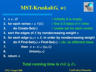
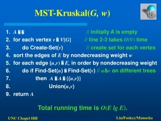
MST-KRUSKAL(G,w) 1. A 2. for each vertex v V[G] 3. do MAKE-SET(v) 4. sort the edges of E by nondecreasing weight w 5. for each edge (u,v) E, in order by nondecreasing w 6. do if FIND-SET(u) FIND-SET(v) 7. then A A {(u,v)} 8. UNION(u,v) 9. return A
Analysis • Initialization O(V) • Sort of edges O(E lg E) • O(E) disjoint forest operations • total time O(E(E,V)) • (E,V)=O(lg E) O(1) O(E) • Total time O(E lg E)
Implementation of Prim’s Algorithm • Management of a priority Q is the critical step in Prim’s algorithm • Can use a binary heap for the Q • Theoretical performance can be improved by using Fibonacci heap • In practice, binary heaps are usually better
MST-PRIM(G,w) 1. A V[G} 2. for each vertex u Q 3. do key[r] 4. key[r] 0 5. [r] nil 6. while Q 7. do u EXTRACT-MIN(Q) 8. for each v Adj[u] 9. do if v Q and w(u,v) < key[v] 10. then [v] u 11. key[v] w(u,v) 12. return A
Analysis of Prim’s • Q as a binary heap • BUILD-HEAP O( ) • While loop executed ? times • for loop within while loop O( ) • test for membership in Q in line 9 • assignment in line 11 has implicitly DECREASE-KEY O( ) • Total time O( ) = O( )