Download
1 / 32
320 likes | 445 Views
Fat Curves and Representation of Planar Figures. L.M. Mestetskii Department of Information Technologies, Tver’ State University, Tver, Russia Computers & Graphics 24 (2000) Computer graphics in Russia. Outline. Abstract Fat curves Boundaries of fat curves

E N D
Fat Curves and Representation of Planar Figures L.M. Mestetskii Department of Information Technologies, Tver’ State University, Tver, Russia Computers & Graphics 24 (2000)Computer graphics in Russia
Outline • Abstract • Fat curves • Boundaries of fat curves • Implicit representation of fat curves • Direct rasterization of fat curves • Engraving representation • Approximation of an engraving by fat Bezier curves
Abstract • Fat curve = “curve having a width” • trace left by a moving circle of variable radius • Engraving • union of a finite number of fat curves • Goal • Bezier representation for fat curves • 2D modeling through engraving • approximation of arbitrary bitmap binary images
Problem • Transforming the engraving representation into a discrete one in order to render a figures on raster display devices (Inverse Problem) • Obtaining an engraving representation of figures given by their discrete or boundary representation
Method • Bezier performance of greasy lines • Decomposition of fat curves on parts with simple envelopes • Scan-converting of fat curves based on Sturm polynomials • Representation of any binary image as fat curves on the basis of its continuous skeleton
P(u,v) r (x,y) Fat Curves • Set of circles in the Euclidean plane R2C: [a, b] → R2× [0, ∞) , t∈[a, b]Ct= {(x, y): (x−u(t))2+(y−v(t))2 ≦ (r(t))2, (x,y)∈R2} • Fat curve • C = ∪t∈[a,b]Ct • axis: P(t) • width: r(t) • end circle: Ca, Cb(initial and final circles) • may be considered as the trace of moving the circle Ct
Example of a Fat Curve • Planar Bezier curve • a set of circles on the plane: H = {H0,H1,…,Hm} • circle Hi, radius Ri, Center (Ui, Vi), i = 0,…,m [Bernstein polynomials]
H2 H3 H1 H4 H5 H0 H6 Example of a Fat Curve • axis: P(t) = (u(t),v(t)), width: r(t) • axis P(t) is an ordinary Bezier curve of degree m with the control points formed by the centers of the circles from H • control circles: H0, H1,…, H6 • control polygon: H 21 circles of family Ct(t = 0.05j, j = 0,…,21)
Boundaries of Fat Curves • A family of circles • Under certain conditions, the family of circles, which is a family of smooth curves, has an envelope curve • The necessary conditions for a point (x,y)∈R2 to the envelope of a family of curves given by the equation F(x, y, t) = 0
(x2,y2) (x1,y1) Find the Envelope Curve the first condition is always satisfiedthe second condition can be violated(no envelopes) Condition:
(x2,y2) (x1,y1) Find the Envelope Curve • A parametric description of two envelopes • Define
Envelopes • Consider in more detail the case when the condition is violated and envelopes do not exist • Interval on which is found as a result of the decomposition of a fat curve
exterior envelope interior envelope (u,v) (x,y) r exterior envelope exterior envelope Envelopes • Consider a fat curve for which envelopes exist • An envelope of a family of circles can be exterior of interior (don’t belong to the boundary of the fat curve) • Criterion for distinguishing interior envelops • direction of axis : (u’, v’) • direction of envelope : (x’, y’) • exterior (supporting orientation) : u’x’ + v’y’ > 0 • interior (opposing orientation) : u’x’ +v’y’ < 0
Envelopes • An envelope can change its orientation from supporting to opposing and conversely • x’ = y’ = 0 • cut a fat curve at point t∈[a, b] where x’=y’=0, we obtain fat curves with constantly oriented envelopes
v’=0 u’=0 Envelopes • Two-side fat curve: both envelopes are exterior • when envelopes are self-intersecting or intersect each other, it must be decomposed into parts • to find monotonicity intervals: u’(t) = 0 or v’(t) = 0 • One-side fat curve: one of the envelopes is interior
v’=0 exterior envelope u’=0 (u,v) (x,y) r exterior envelope Rules for Decomposing Fat Curves • Three rules for decomposing fat curves • separate fat curves for which u’2+v’2 >= r’2 • separate one-side fat curves by finding singular points of envelopes, i.e., points where x’1=y’1=0 or x’2=y’2=0 • Separate monotone fat curves by finding points for which u’=0 or v’=0
Implicit Representation of Fat Curves • Membership function of the set • point belongs to the fat curve if the following condition is satisfied for a certain
Direct Rasterization of Fat Curves • The discrete tracing of contour of a domain given by its membership function consists in an inspection of the points with integer coordinates located along this contour
Engraving Representation of a Binary Image • Obtain a continuous representation of a figure given by its discrete representation • The solution of this problem involves 3 steps • approximate the given bitmap binary image by a polygonal figure (PF) • construct a skeletal representation of the PF • approximate the skeletal representation of the PF by fat curves
Polygonal Figure • Each of the PF is a polygon of the minimum perimeter that separates the black and white pixels of the bitmap image • Problem • constructing an engraving representation of the given bitmap image • construction of an engravingrepresentation of the PF polygonal figure of the minimum perimeter
Skeletal Representation • Consider the set of all circles in the plane • all their interior point are also interior of the PF • the boundary of each circle at least two boundary points of the PF • circles: inscribed empty circles • set of centers of such circles forms the skeleton of the PF • skeletal representation of a bitmap image: skeleton + inscribed empty circles
Sites & Bisector • PF consists of vertices and segments: sites • every empty circle touches two or more sites • The maximal connected set of the centers of the inscribed empty circle that touch these sites: bisector of a pair of sites • a segment of a line or a segment of a parabola
Sites & Bisector • Askeleton is an almost complete engraving • There possible combinations of the pairs of sites • segment-segment, point-segment, point-point • Segment-segment
Sites & Bisector • Point-segment find z, follows from that since and, hence,
Sites & Bisector • Point-point • The engraving constructed on the basis of the skeletal representation of a PF will be called the skeletal engraving
Approximation of an Engraving by Fat Bezier Curves • Skeletal engravings provide a highly accurate description of bitmap binary images (too many fat curves) • Considered as a problem of the approximation of a skeletal engraving G by another engraving G’ • The Hausdorff metric may be conveniently measure the distance between engravings • Find an engraving G’ such that
Branch • Skeleton structure • juncture vertices of degree 3 or higher • terminal vertices of degree 1 • intermediate vertices of degree 2 • A chain of edges that have common vertices of degree 2 will be called a branch • The entire skeleton can be represented as the union of such branches
Approximation • Consider a chain of n fat curves C1,…,Cn corresponding to the same branch of the skeleton • find a fat curve C in a certain class of fat curves that provides the best approximation for this sequence of circles • e.g., in the class of cubic Bezier curves C∈B3 • in other word, we must solve the minimization problem
Fat Curve Fitting Problem • Empty circles K0,…Kn located at the vertices of the branch • Define
Fat Curve Fitting Problem • The approximation fat curve C is sought in the form of a Bezier curve of degree mH0,…,Hm are the control circles of C(t) • The problem is to find a set of control circles such that it minimizes the quadratic mean distance from the empty circles K0,…,Kn
Fat Curve Fitting Problem • In the optimization problem, the objective function • The optimal solution if found by solving a system of linear equations obtained from the following condition: • If the fat Bezier curve with the control circles H0,…,Hm does not provide the desired accuracy • the chain of n fat curves C0,…,Cm is partitioned into two shorter chains, and the approximation problem is solved separately for each of these chains