Download
1 / 30
310 likes | 444 Views
Multi-scale Simulation of Wall-bounded Flows. Ayse G. Gungor and Suresh Menon Georgia Institute of Technology Atlanta, GA, USA Supported by Office of Naval Research WALL BOUNDED SHEAR FLOWS: TRANSITION AND TURBULENCE Isaac Newton Institute for Mathematical Sciences Cambridge, UK

E N D
Multi-scale Simulation of Wall-bounded Flows Ayse G. Gungor and Suresh Menon Georgia Institute of Technology Atlanta, GA, USA Supported by Office of Naval Research WALL BOUNDED SHEAR FLOWS: TRANSITION AND TURBULENCE Isaac Newton Institute for Mathematical Sciences Cambridge, UK September 11th, 2008
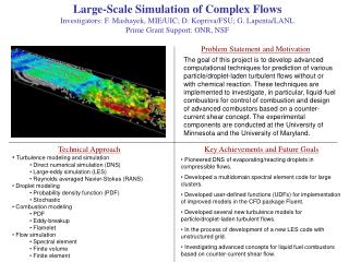
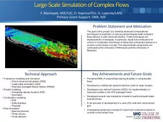
Flows of engineering relevance is at high Re Wall bounded flows, wake and shear flows The cost of simulations that resolve all the scales of motion is of the order of Re3 Almost 90% of this cost is a result of attempting to explicitly resolve near-wall boundary layers Near-wall turbulence contains many small, energy containing, anisotropic scales that should be resolved DNS Computations of channel flows 18 B grid points, Ret= 2003 (Hoyas et al., 2006) DNS Computations of turbulent separated flows 151 M grid points, Ret = 395 (Marquillie et al., 2008) DNS at lower Reynolds number (Experiment at Ret= 6500) Motivation
Conventional LES requires very high near-wall resolution Near-wall Models Use algebraic relationships to compute wall stresses Resolution requirement reduced significantly Additional source of errors due to the modeling the dynamics in the near-wall region Zonal Approaches Two Layer Approach – Solves boundary layer equations and/or employ local grid refinement RANS-LES Approach – Uses RANS near the wall and LES in the core region Most of the cost-effective approaches do not properly resolve the turbulent velocity fluctuations near the wall Here, a two-scale approach for high-Re flows is discussed attempts to resolve near-wall fluctuations Motivation
Multi-Scale Simulation Approaches Multi-scale approaches: Dynamic multilevel method (Dubois, Temam et al.) Rapid Distortion Theory SS model (Laval, Dubrulle et al.) Variational multiscale method (Hughes et al.) Two-level simulation (TLS*) (Kemenov & Menon), extended for compressible flows (Gungor & Menon) Simulate both LS and SS fields explicitly Computed SS field provides closure for LS motion All use simplified forms of SS equations Some invoke eddy viscosity concept for SS motions TLS simulates the SS explicitly inside the LS domain *Kemenov and Menon, J. Comp. Phys., Vol. 220 (2006), Vol. 222 (2007) Gungor and Menon, AIAA-2006-3538
Two-Level Simulation: Key Features Simulate both large- and small-scale fields simultaneously large-scales (LS) evolve on the 3D grid small-scales (SS) evolve on 1D lines embedded in 3D domain 3D SS equations collapsed to 3x1D equations with closure Scale Separation approach employed No grid or test filtering invoked No eddy viscosity assumption invoked High-Re flows simulated using a “relatively” coarse grid Efficient parallel implementation needed Cost becomes acceptable for very high-Re flow Potential application to complex flows
Large-Scale Grid DyLES DzSS DxSS Small-Scale Grid y x z DySS DzLES DxLES Two Level Grid in the TLS-LES Approach Small scale equations are solved on three 1D lines embedded in the 3D domain Resolution requirements • Number of LES control volumes: NLES3 NLES <NSS • Grid points for TLS-LES: NLS3 + 3NLS2NSS NLS <NLES, NLS <<NSS • Grid points for DNS: NSS3
TLS v/s LES Two degrees of freedom in Conventional LES Filter Width and Filter Type Two degrees of freedom in TLS: Sampling/Averaging Operator (SS <=> LS) Interpolation Operator (LS <=> SS) TLS does not require commutativity to derive LS Eqns. Full TLS approach described earlier isotropic turbulence, free shear and wall-bounded flows* Here, a new hybrid TLS-LES approach demonstrated** Application to wall bounded flows with separation * Kemenov and Menon, J. Comp. Phys. (2006, 2007) ** Gungor et al., Advances in Turbulence XI (2007)
TLS – Scale Separation Operator L Exact Field is split into LS and SS fields: Continuous large scale field is defined by adopted LS grid: Sampling at LS grid nodes Interpolation to the SS nodes SS field is defined based on LS field from decomposition:
A priori analysis of scale separation operators (LES and TLS) Fully resolved signal (black) from a 1283 DNS of isotropic turbulence study. The resolved field is represented with a 16 grid point. The top hat filtered LES field (red) obtained by taking a moving average of the fully resolved field over 8 points. The TLS LS field (green) truncated from the fully resolved signal. The TLS SS field (blue) obtained by subtracting the LS field from the fully resolved field. TLS has higher spectral support The longitudinal energy spectra of a fully resolved signal (black) and (a) LES energy spectra (red), (b) The TLS LS (green) and SS (blue) energy spectra.
The TLS equations are used in the near-wall region The LES equations are used in the outer flow All zonal approaches (Hybrid RANS-LES) use some form of domain decomposition Hybrid TLS-LES uses functional decomposition No need for interface boundary conditions Need to determine the transition region dynamically LES LES prescribed y interface for wall-normal lines prescribed y interface TLS RANS Hybrid RANS-LES Strategy TLS-LES Strategy Hybrid TLS-LES Wall Model
Hybrid TLS-LES scale separating operator Rdefined as an additive operator that blends the LES operator F with the TLS operator L R= k F + (1 - k) L LES operator F is the standard filtering operator k is a transition function relating TLS and LES domains Hybrid TLS-LES Formulation – Scale Separation Step Function Tanh Function
Application of additive scale separation operator Velocity components Turbulent stress Hybrid TLS-LES Equations Hybrid Terms • Hybrid terms also in RANS-LES formulation (Germano, 2004) • Combination of time and space operation • Here, the hybrid terms appear due to LES and TLS combination • both are space operators !!
Resolved / Large Scale Equations Hybrid TLS-LES Equations Continuity: Momentum: The unresolved term in the momentum equation LES: any SGS model Specific closures for each model TLS: The scale interaction terms are closed if the small scale field is known
Small Scale Equations Represents the smallest scales of motion “Hybrid TLS-LES SS domain” discrete set of points along 3- 1D lines 3D evolution of small-scales in each line Full 3D SS equations “collapsed” on to these 1D lines Cross-derivatives modeled based on a priori DNS analysis Channel and forced isotropic turbulence (Kemenov & Menon, 2006, 2007) Explicit forcing by the large scales on these 1D equations Hybrid TLS-LES Equations Continuity: Momentum:
Numerical Implementation of SS Equations 1) Approximate LS field on each 1D SS line by linear interpolation 2) Evolve SS field from zero initial condition until the SS energy matches with the LS energy near the cut off 3) Calculate the unclosed terms in the LS equation Time evolution of the SS velocity and SS spectral energy
Hybrid TLS-LES of Channel Flow • Mean velocity profiles demonstrates the capability of the model • Wall skin friction coefficient provides • good agreement with DNS • well comparison with Dean’s correlation
Ret = 590 Ret = 2400 Ret = 1200 Hybrid TLS-LES of Channel Flow 3-D energy spectra Hybrid TLS-LES approach recovers both LS and SS spectra near the wall Red line : Instantaneous energy spectra Blue line : Volume average spectra Black line: k-5/3 slope
Incompressible Multi-domain Parallel Solver 4th order accurate kinetic energy conservative form (used here) 5th order accurate upwind-biasing for convective terms 4th order accurate central differencing for the viscous terms Pseudo-compressibility with five-stage Runge – Kutta time stepping Implicit time stepping in physical time with dual time stepping DNS, LES (LDKM), TLS-LES Numerical Solver
Turbulent Channel Flow • Coarse DNS – 192 x 151 x 128 • Well prediction of the mean velocity, turbulent velocity fluctuations and turbulent kinetic energy budget.
Hybrid TLS-LES of Separated Channel Flow • Hybrid TLS-LES(~0.18M) and LES(~1.6M) at Ret = 395 • DNS(~151 M) at Ret = 395 by Marquillie et al., J. of Turb., Vol. 9, 2008 • Experiment at Ret = 6500 by Bernard et al., AIAA J., Vol. 41, 2003 • Spatial resolution (%75 coarser than DNS) • TLS-LES-LS (64 x 46 x 64) : Dx+LS = 77.4, Dz+LS = 19.2, Dy+LS = 5.4 • TLS-LES-SS (8 SS points/LS): Dx+SS = 9.6, Dz+SS = 2.4, Dy+SS = 0.68 • DNS (1536 x 257 x 384) : Dx+ = 3, Dz+ = 3, Dy+|max = 4.8 • Inflow turbulence from a separate LES channel study at Ret = 395 Total vorticity on a spanwise plane (LES) Streamwise vorticity on a horizontal plane (LES)
Time evolution of the SS velocity Spanwise line in the separation region
SS evolution effect on the instantaneous flow SS iterations: 20 SS iterations: 100 • simulations on each line • optimal parallel approach SS iterations: 300 SS vorticity magnitude isosurfaces colored with SS streamwise velocity
Hybrid TLS-LES of Separated Channel Flow • Hybrid TLS-LES grid is chosen very coarse deliberately • Hybrid TLS-LES Cp shows good agreement with DNS • ~%30 off from experiments (higher Re) for all studies • Hybrid TLS-LES Cf in reasonable agreement with DNS and LES • Separation is not properly predicted due to coarse LS resolution
Hybrid TLS-LES of Separated Channel Flow Streamwise velocity fluctuation Wall-normal velocity fluctuation DNS-151M (circles and shaded contours), TLSLES (red), LES (green) The authors would like to thank Dr. J.-P. Laval for providing the DNS data
Hybrid TLS-LES of Asymmetric Diffuser Flow • Hybrid TLS-LES(~0.25M) and LES(~1.8M) at Ret = 500 • LES(~6.5 M) by Kaltenbach et al., J. of Fluid Mech., Vol. 390, 1999 • Experiment by Buice and Eaton, J. of Fluids Eng., Vol. 122, 2000 • The main features of this flow • A large unsteady separation due to the APG • A sharp variation in streamwise pressure gradient • A slow developing internal layer • Inflow turbulence from a separate LES channel study at Ret = 500 Inclination angle: 100
TLS LES TLS Hybrid TLS-LES of Asymmetric Diffuser Flow • Spatial resolution • TLS-LES-LS (110 x 56 x 40) : Dx+LS = 54, Dz+LS = 50, Dy+LS = 5.72 • TLS-LES-SS (8 SS points/LS) : Dx+SS = 6.7, Dz+SS = 6.2, Dy+SS = 0.72 • LES (278 x 80 x 80) : Dx+ = 25, Dz+ = 25, Dy+ = 0.98 • LES by Kaltenbach et al., 1999 (590 x 100 x 110) • Step function ( , F: LES, L: TLS operator) • pre-defined interface, Y+TLS = 152 Isosurfaces of the second invariant of the velocity gradient tensor colored with local streamwise velocity predicted with LES model
Hybrid TLS-LES of Asymmetric Diffuser Flow • Cp along the lower and upper wall predicted reasonably well • Hybrid TLS-LES shows reasonable agreement with the experiment • Skin friction coefficient over the upper flat wall displays a strong drop and a long plateau starting near the separation region in the bottom wall, and a more gradual decrease downstream • Overall, TLS-LES shows ability to predict separation regions without any model changes
Hybrid TLS-LES of Asymmetric Diffuser Flow • The total pressure decreases 30% in the streamwise direction due to frictional losses. • Mean velocity predicted reasonably with the hybrid TLS-LES model • Separation location agrees well • But reattachment is observed further downstream Exp. (symbols), TLS-LES (dashed lines) LES (solid lines)
A generalized hybrid formulation developed to couple TLS-LES New hybrid terms identified but they still need closure TLS as a “near-wall” model for high-Re flows used in a TLS-LES approach without the hybrid terms Reasonable accuracy using “relatively” coarse LS grid Potential application to complex flows with separation Efficient parallel implementation can reduce overall cost Conclusion and Future Plans Next Step • Analyze the hybrid terms in the TLS-LES equations and develop models for hybrid terms • A priori analysis of SS derivatives for arbitrarily positioned SS lines