Download
1 / 17
180 likes | 386 Views
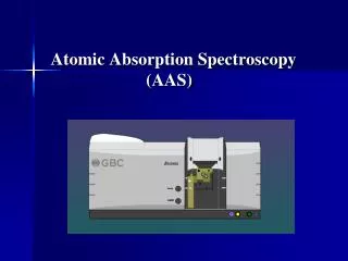
Atomic Absorption Spectroscopy AAS. Comparatively easy to use Low maintenance Low consumables Good for measuring one element at a time. Block Diagram. h n + M → M* Sample is vaporized/atomized by: Flame Electrothermal Vaporizer (ETV). AA Sources- HCL.

E N D
Atomic Absorption SpectroscopyAAS Comparatively easy to use Low maintenance Low consumables Good for measuring one element at a time.
Block Diagram hn + M → M* Sample is vaporized/atomized by: Flame Electrothermal Vaporizer (ETV)
Flame AAS: sample introduction Sample is dissolved into solution (usually acidic). Sample is pulled through straw into nebulizer. Most of samples goes to waste. Nebulizer sends droplets/aerosol to flame to be de-solvated, resulting in gaseous molecules/atoms.
To excited free atoms, flame must break any molecules apart into discrete atoms. Potential Problems: Atoms recombine readily in flame, especially with O2. If flame is too energetic, ionization of atoms can occur - won’t be detected. MX (g)→ M (g) + X(g) M + O → MO M → M+ + e- Flame processes
Burner Head want a long optical pathlength.
Electrothermal Vaporization First demonstrated in 1961 by L'vov (USSR) Use electrically heated carbon furnace Excellent LOD More sensitive than flame: Entire sample atomized at once Residence time of vapor in optical path >1 s Potential problem: poor precision due to sampling variability LOD for Mg Flame: 0.1 ppm ETV: 0.00002 ppm - 20 pptr
Cold Vapor (CV) Atomization Mercury Reduced by SnCl2
Physical Interferences Droplet size from nebulizer depends on surface tension of solution. Organic solvent (alcohol, ester, ketone) can lead to smaller droplets, more intense signal.
Chemical Interferences Formation of compounds of low volatility, ex. CaSO4 Ionization M M+ + e- Add ionization suppressors - create electron-rich environments. Ex, alkali metals
Spectral Interferences Two or more lines within monochromator’s spectral bandpass - requires appropriate resolution from diffraction grating (line spacing)
Double-Beam Instrument A reference beam is used as a “blank” signal. To get %T measurement, you have to know what the measurement for 100% T is. Because the flame is always fluctuating, we need the reference beam to give a point of reference at any time during experiment - compensates for “drift”.
Background Correction Flame creates a messy background - scattering, absorbance by molecular species (oxides, hydroxides) Another wavelength is passed through the flame, its %T measured. Any loss of T is due to scattering, losses unrelated to absorption by analyte. The analyte %T is corrected for these losses.
Atomic Fluorescence Spectroscopy • Fundamental Process • hn + M → M* → M + hn' • Photon emitted is not the same energy as the photon absorbed – it has lower energy • fluorescence signal is directly proportional to concentration • Enhanced sensitivity over AAS • Signal collected at 90° angle - avoid having to filter out source radiation Fluorescence
Quantitative Analysis - Calibration Curve Test a series of standards and plot Abs v. conc, find LDR Run your sample and determine conc with line equation. ppm = g/mL ppb = ng/mL For aqueous solutions (~1 g/mL)
Quantitative Analysis - Standard Additions Method Spike your standards into your samples - it’s all the same matrix. cx = bcs/mVx S = standard X = unknown From graph : Cx = -(x-int)*cs/Vx