Download
1 / 25
250 likes | 316 Views
The Dirac operator spectrum from a perturbative approach. F. Di Renzo M. Brambilla, M. Dall’arno. Università di Parma and INFN, Parma, Italy. Disclaimer : this is work in progress ….

E N D
The Dirac operator spectrum from a perturbative approach F. Di Renzo M. Brambilla, M. Dall’arno Università di Parma and INFN, Parma, Italy
Disclaimer: this is work in progress … My own expertise has been for quite a long time in a (non diagrammatic) way of doing Lattice Perturbation Theory. I have to warn you that this is still another application of NSPT! In what follows I collect mainly ideas and very preliminary results: this is really work in progress. Still, I think there’s already some flavour of what we aim at. Let’s have a very first glance
Outline • Preludio: the spectrum of the Dirac operator as a probe for • chiral (and deconfinement ?!) transition. • Polyakov loop, Z(3),different boundary conditions and all that... • A skecth of the technique by which computations were made (NSPT): • from Stochastic Quantization to Stochastic Perturbation Theory • from SPT to Numerical SPT • The case of Lattice Gauge Theories and different vacua. • The computation of the spectrum: • a degenerateeigenvalue problem in Perturbation Theory • Very preliminary results: where do the Dirac eigenvalues accumulating near zero come from? • Our spectra are highly degenerate: do we need a regulator? • Outlook
The Dirac spectrum: why The transition associated to chiral symmetry breaking has a natural order parameter and this is connected to the Dirac operator spectrum (Banks and Casher, 1980). This made the Dirac eigenvalue density (which is not a natural observable in Field Theory) a natural quantity to be interested in. What does spontaneous chiral symmetry breaking actually mean? (Verbaarschot) A small quark mass leads to a macroscopic reallignement of the QCD vacuum. Since we are led to look for an accumulation of Dirac eigenvalues near zero (otherwise a small quark mass would be dominated by much larger eigenvalues). Defining the density of eigenvalues the relation we are looking for was put forward by Banks and Casher. The chiral condensate (the order parameter of the transition at hand) can be expressed as
The small eigenvalues we are looking for are not there in the free case (deep perturbative, chirally simmetric regime). So, they must be due to the interaction mediated by gauge fields. As a matter of fact, any interaction in quantun mechanics produces a repulsion among eigenvalues and this is a natural mechanism to account for the rearrangement we are after. This is actually one natural candidate for the Physics of Banks Casher: eigenvalues sitting near zero are coming from the bulk. (Not the only candidate: istantons contributions?) • With this respect Perturbation Theory is in a tantalizing situation • On one side, it sits (deep!) in the chirally symmetric phase, while we are after an effect (non zero eigenvalue density in the low end of the spectrum) which lives at its boundary! • On the other side, repulsion among eigenvalues is a phenomenon we can typicall inspect in PT! (canonical example is level splitting in non-relativistic QM)
We will compute the spectrum of D†D in PT (plain Wilson fermions). • We start our journey with some no-go barriers standing on our way: • We sit (deep!) in the chirally restored regime while we look for a way to get to its frontier… • We are aware of the asymptotic nature of any perturbative expansion… • We deal with Wilson fermions (ok… well… chiral properties not so brilliant…) • We can nevertheless hope to turn (at least part) of the difficulties into opportunities: • It is interesting enough to understand how far PT can lead us towards chiral symmetry breaking (coming from the other side!) • We can get some piece of information from the (at least apparent) convergence properties of an asymptotic perturbative expansion. • We can hope to follow the eigenvalues in their way to zero!
As a matter of fact spectral observables are not that natural as objects (observables?) in Quantum Field Theory. Define the average number of eigenvalues of Dm†Dmwithin a given threshold Then consider the spectral sums defined as (it is sufficient to understand their renormalization properties because one can invert to get mode number) It turns out that these spectral sums can be mapped to composite operators in Twisted Mass QCD, in terms of which they have a natural renormalization prescription (renormalize all the masses which are around with ZP…) Take care of spectral observables renormalization properties! (M. Luscher, L. Giusti). Dealing with Wilson fermions, in our case we also have to care of critical mass counterterms.
A few years ago Gattringer put forward a relation between Polyakov loop and Dirac spectrum in the background of different Z(3) vacua. In his more recent words, “the response of Dirac spectra to different temporal boundary conditions contains information about confinement”. Polyakov loop, Z(3) and all that… Are spontaneous chiral symmetry breaking and confinement in the end related? The relation beween chiral symmetry breaking and confinement is one the long standing problem of our field. As the chiral condensate is an order parameter for the first transition, Polyakov loop is for sure related to the second. The Polyakov loop is an order parameter for the quenched case, in which Z(3) symmetry and its breaking are in place. Due to its relation to static quark-antiquark potential, it is a good indicator for confinement also for the complete theory. • Our idea: compute the Dirac spectrum in the background of different Z(3) vacua. • Is the repulsion of eigenvalues much the same? • How do convergence properties of the series compare? • How does the reconstruction of Polyakov loop work in perturbation theory?
Stochastic Quantization and Stochastic Perturbation Theory Given a field theory, Stochastic Quantization basically amounts to giving to the field an extra degree of freedom, to be thought of as a stochastic time in which an evolution takes place according to the Langevin equation In the previous formula, h is a gaussian noise, from which the stochastic nature of the equation originates. Now, the main assertion is very simply stated: asymptotically From Stochastic Quantization to NSPT NSPT comes almost for free from the framework of Stochastic Quantization (Parisi and Wu, 1980). From the latter originally both a non-perturbative alternative to standard Monte Carlo and a new version of Perturbation Theory were developed. NSPT in a sense interpolates between the two.
And hereStochastic Perturbation Theory comes Without entering into details: solve by iteration … Diagrammatically ... ... and this is a propagator ... + λ + λ2 ( + ... ) + O(λ3) ) + O(λ2) + 3 λ ( + To understand, take the standard example: f4 theory ... The free case is easy to solve in term of a propagator ... ... and for the interacting case you can always trade the differential equation for an integral one ...
Numerical Stochastic Perturbation Theory Since the solution of Langevin equation will depend on the coupling constant of the theory, look for the solution as a power expansion If you insert the previous expansion in the Langevin equation, the latter gets translated into a hierarchy of equations, each for each order, each dependent on lower orders. Now, also observables are expanded Observation: we can get power expansions from Stochastic Quantization’s main assertion, e.g. NSPT (Di Renzo, Marchesini, Onofri 94) simply amounts to the numerical integration of SPT equations on a computer! Of course this time we are dealing with a LATTICE regularization in x-space and the time evolution has of course to be discretized ...
NSPT for Lattice Gauge Theories (JHEP0410:073) Langevin equation for LGT goes back to the 80’s (Cornell Group 84): the main point is to formulate a stochastic process in the group manifold. Then one has to implement a finite difference integration scheme (i.e. Euler)
NSPT around non trivial vacua 1 is not the only trivial order for our expansion! Other vacua are viable choices as well! Uxm(0)(t;h) Since dynamics is dictated by the equations of motion, any classical solution is good enough!
Fermionic observables are then constructed by inverting (maybe several times) the Dirac matrix on convenient sources. The Dirac matrix in turn is a function of the gluonic field, and because of that is expressed as a series as well The good point is that free part is diagonal in p-space, while interactions are diagonal in x-space: go back and forth via FFT! This is also crucial in taking into account fermions in the evolution.
On the (perturbative) configurations we produce via NSPT dynamics we want to compute something like (a very general notation) Our goal is to get the perturbative solutions We express the solution in terms of projectors inside and outside the degeneration space of the starting (unperturbed, i.e. free field) eigenvalue. Notice that inside the free field eigenspace there is the component selected by diagonalizing the perturbation and a component perpendicular to it. Degenerate eigenvalues PT A textbook computation … still many textbooks mess up with it!
Results now follow by applying the projectors to the eigenvalue equation We then rewrite our equation • Notice that one recognizes the standard features of perturbative eigenvalues: • Construction is iterative (by the way, our iterative inversion procedure is in place). • Eigenvalues repel each other! Beware! This works if degeneracy is lifted at first order. Otherwise one has to go for a different formalism (i.e. there is a third projector to be taken into account)
Some results Plots are always instructive to look at when you deal with distributions The first (trivial) order (g) of the correction to the second eigenvalue (ordering refers to unperturbed spectrum, i.e. free field)
The first non trivial order (g2) of the correction to the second eigenvalue (ordering refers to unperturbed spectrum, i.e. free field)
Now it is good to go back to our movie: this is density of eigenvalues up to one loop, lowering from 40 to 6 (on a 64 lattice)
We plot the plain value of the eigenvalues (ordered at tree level). Red is tree level, black is correction at one loop (44) Where do eigenvalues moving to zero come from? Plots are always instructive to look at when you deal with distributions
Is it an artifact? Always look for finite volume effects … Again. Red is tree level, black is correction at one loop (64)
Once again it is good to go back to a movie: let’s have a look at the repulsion
Distributions for higher loops display hugetails! Why only one loop? NSPT is there to go higher than that …
A consistency check was performed by computing both directly and via the eigenvalues quantitites like Remember: Now, if degeneracy is still there at first order, one has to look for Is there anything going really wrong? Always check results, if you can … It was ok! Notice that there is a potential source of numerical instability which is easy to spot and we are now trying to investigate: The dimension of degenerate eigenspaces at tree level can be large; if by numerical artifacts one misses a residual degeneracy, the effect is going to be huge! IDEA: use it as a regulator when first order corrections almost coincide…
Conclusions • I only discussed preliminary results. • There is something already valuable: one can really see that eigenvalues repulsion is indeed there (and they come from the bulk to zero). • We now should try to understand what is going on at higher loops. • Computations in the background of different Z(3) vacua are under their way. • Having the whole spectrum at disposal opens the way to a variety of computations…