Download
1 / 21
210 likes | 548 Views
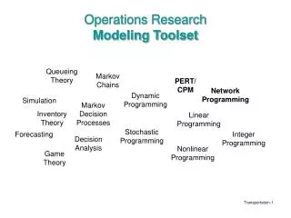
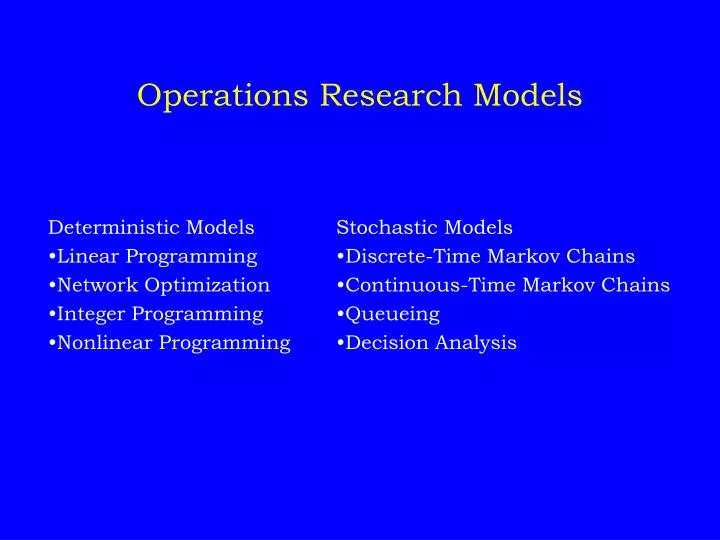
Operations Research Models. Deterministic Models Stochastic Models •Linear Programming •Discrete-Time Markov Chains •Network Optimization •Continuous-Time Markov Chains •Integer Programming •Queueing •Nonlinear Programming •Decision Analysis . Deterministic Models.

E N D
Operations Research Models Deterministic Models Stochastic Models •Linear Programming •Discrete-Time Markov Chains •Network Optimization •Continuous-Time Markov Chains •Integer Programming •Queueing •Nonlinear Programming •Decision Analysis
Deterministic Models Most of the deterministic OR models can be formulated as mathematical programs. "Program" in this context, refers to a plan and not a computer program. Mathematical Program Maximize / minimize z = f(x1, x2, . . . , xn) subject to gi(x1, x2, . . . , xn) = bi, i = 1,…,m xj 0, j = 1,…,n
Notation xj= decision variables (under control of decision maker) f(x1, x2, . . . , xn) = objective function gi(x1, x2, . . . , xn) = bi, structural constraints or technological constraints (may be written as inequalities: or xj 0, nonnegativity constraints • Feasible solution: vector x = (x1, x2, . . . , xn) that satisfies all the constraints. • Objective function ranks all feasible solutions
Linear Programming A linear program is a special case of a mathematical program in which all the functions are linear: Maximize z = c1x1 + c2x2 + . . . + cnxn subject to a11x1 + a12x2 + . . . + a1nxn = b1 a21x1 + a22x2 + . . . + a2nxn = b2 : : am1x1 + am2x2 + . . . + amnxn = bm xj uj, j = 1,…,n xj 0, j = 1,…,n
Linear Programming Notation xj ujare called simple bound constraints x = decision vector (activity levels) cj,aij, bi, ujare all known data Goal find x
Linear Programming Assumptions ( i) Divisibility (ii) Proportionality Linearity (iii) Certainty
Explanation of Assumptions (i) Divisibility: fractional values for decision variables are permitted. (ii) Proportionality: contribution of activity j to (a) objective function = cjxj (b) constraint i = aijxj Both are proportional to the level of activity j. No cross-terms can appear in the model; e.g., 3x1x2. Volume discounts, setup charges, and nonlinear efficiencies are similarly not permitted.
(iv) Certainty: the data cj,aij, bi, uj are known and deterministic. • Note: • Integer or nonlinear programming must be used when either assumption (i) or (ii) cannot be justified. • Stochastic models must be used when a problem has significant uncertainties in the data that must be taken into account in the analysis.
Example Q P Machines: A, B, C, D $ 9 0 / unit $ 1 0 0/ unit Available times differ 40 unit/wk 100 unit/wk Operating expenses not including raw materials: $3000/week D 15 min/unit D 10 min/unit P ur c has e P a rt $5 / U C 9 min/unit C 6 min/unit B 16 min/unit A 20 min/unit B 12 min/unit A 10 min/unit R M 1 R M 3 R M 2 $ 2 0 / U $ 2 0 / U $ 2 0 / U
Data Summary P Q Selling price/unit 90 100 45 40 Raw Material cost/unit 100 40 Demand (maximum) 20 10 mins/unit on A 12 28 B 15 6 C D 10 15 Machine Availability: A 1800 min/wk; B 1440 min/wk, C 2040 min/wk, and D 2400 min/wk Operating Expenses = $3000/wk (fixed cost) Decision Variables xP = # of units of product P to produce per week xQ = # of units of product Q to produce per week
x Q Model Formulation = z Objective function 45 + 60 Maximize subject to x x p Q £ 20 + 10 1800 x x Structural p Q £ constraints 12 + 28 1440 x x p Q £ 15 + 6 2040 x x p Q £ 10 + 15 2400 x p demand xP £ 100, xQ£ 40 Are we done? xP³ 0, xQ³ 0 nonnegativity Optimal solution Are the LP assumptions valid for this problem? xP* = 81.82, xQ* = 16.36 z* = 4664
Graphical Solutions to LPs Linear programs with 2 decision variables can be solved with a graphical procedure. • Plot each constraint as an equation and then decide which side of the line is feasible (if it’s an inequality). • Find the feasible region. • Plot two iso-profit (or iso-cost) lines. • Imagine sliding the iso-profit line in the improving direction. The “last point touched” in the feasible region when sliding iso-profit line is optimal.
Solution to Production Planning Problem • Optimal objective value is $4664 but when $3000 in weekly operating expenses is subtracted, we obtain a weekly profit of $1664. • Machines A & B are being used at their maximum levels and are bottlenecks. • There is slack production capacity in Machines C & D. • How would we solve model using Excel Add-ins ?
Possible Outcomes of an LP 1. Infeasible – feasible region is empty; e.g., if the constraints include x1 + x2 6 and x1 + x2 7 (no finite optimal solution) 2. Unbounded - Max 15x1 + 15x2 s.t. x1 + x2 1 x1 0, x2 0 3. Multiple optimal solutions - Max 3x1 + 3x2 s.t. x1 + x2 1 x1 0, x2 0 4. Unique optimal solution. Note: multiple optimal solutions occur in many practical (real-world) LPs.
x 2 z z z 2 3 1 4 3 2 1 0 x 0 1 2 3 4 1
z x x Maximize = + 1 2 6 x x subject to 3 + 1 2 x x 3 + 3 1 2 x x 0, 0 1 2 Figure 10. Inconsistent constraint system
Sensitivity Analysis and Ranging Shadow Price (dual variable) on Constraint i Amount object function changes with unit increase in RHS, all other coefficients held constant. RHS Ranges Allowable increase & decrease for which shadow prices remain valid Objective Function Coefficient Ranges Allowable increase & decrease for which current optimal solution is valid