Download

1 / 12
120 likes | 246 Views
Lecture 7. Learning (IV): Error correcting Learning and LMS Algorithm. Outline. Error Correcting Learning LMS algorithm Nonlinear activation Batch mode Least Square Learning. x M (n). w M. d(n) : feedback from environment. u(n). y(n). . w 1. x 1 (n). w 0.

E N D
Lecture 7.Learning (IV):Error correcting Learning and LMS Algorithm
Outline • Error Correcting Learning • LMS algorithm • Nonlinear activation • Batch mode Least Square Learning (C) 2001-2003 by Yu Hen Hu
xM(n) wM d(n): feedback from environment u(n) y(n) w1 x1(n) w0 Supervised Learning with a Single Neuron Input: x(n) = [1 x1(n) … xM(n)]T Parameter: w(n) = [w0(n) w1(n) … wM(n)]T Output: y(n) = f[u(n)] = f[wT(n)xT(n)] Feedback from environment: d(n), desired output. (C) 2001-2003 by Yu Hen Hu
Error-Correction Learning • Error @ time n = desired value – actual value e(n) = d(n) – y(n) • Goal: modify w(n) to minimized square error E(n) = e2(n) • This leads to a steepest descent learning formulation: w(n+1) = w(n) – ' wE(n) where wE(n) = [E(n)/w0(n) … E(n)/wM(n)]T = 2 e(n) [y(n)/w0(n) … y(n)/wM(n)]T is the gradient of E(n) w.r.t. w(n). ’ is a learning rate constant. (C) 2001-2003 by Yu Hen Hu
Case 1. Linear Activation: LMS Learning If f(u) = u, then y(n) = u(n) = wT(n)x(n) Hence wE(n) =2 e(n) [y(n)/w0(n) … y(n)/wM(n)]T = 2 e(n) [1 x1(n) … xM(n)]T = 2 e(n) x(n) Note e(n) is a scalar, and x(n) is a M+1 by 1 vector. Let = 2’, we have the least mean square (LMS) learning formula as a special case of error-correcting learning: w(n+1) = w(n) + h e(n)•x(n) Observation The amount of corrections made to w(n), w(n+1)w(n) is proportional to the magnitude of the error e(n) and along the direction of the input vector x(n). (C) 2001-2003 by Yu Hen Hu
Example Let y(n) = w0(n) •1+ w1(n) x1(n) + w2(n) x2(n). Assume the inputs are: Assume w0(1) = w1(1) = w2(1) = 0, and = 0.01. e(1) = d(1) – y(1) = 1 – [0•1 + 0•0.5 + 0•0.8] = 1 w0(2) = w0(1) + e(1)•1 = 0 + 0.01•1•1 = 0.01 w1(2) = w1(1) + e(1) x1(1) = 0 + 0.01•1•0.5 = 0.005 w2(2) = w2(1) + e(1) x2(1) = 0 + 0.01•1•0.8 = 0.008 (C) 2001-2003 by Yu Hen Hu
Results Matlab source file: Learner.m (C) 2001-2003 by Yu Hen Hu
Case 2. Non-linear Activation In general, Observation: The additional terms is f’ [u(n)]. When this term becomes small, learning will NOT take place. Otherwise, the update formula is similar to LMS. (C) 2001-2003 by Yu Hen Hu
LMS and Least Square Estimate Assume that the parameters w remain unchanged for n = 1 to N (> M). Then, e2(n) = d2(n) 2d(n)wTx(n) + wTx(n)xT(n)w. Define an expected error (Mean square error) Denote Then where R: correlation matrix, : cross correlation vector. (C) 2001-2003 by Yu Hen Hu
Least Square Solution • Solve wE = 0, for W, we have wLS = R1 • When {x(n)} is a wide-sense stationary random process, the LMS solution w(n) converges in probability to the least square solution wLS. LMSdemo.m (C) 2001-2003 by Yu Hen Hu
LMS Demonstration (C) 2001-2003 by Yu Hen Hu
LMS output comparison (C) 2001-2003 by Yu Hen Hu