Download
1 / 26
280 likes | 576 Views
Hamiltonian Chaos and the Ergodic Hypothesis. The Brown Bag Hassan Bukhari BS Physics 2012 墫鱡뱿轺. Stat Mech Project. “ It is not less important to understand the foundation of such a complex issue than to calculate useful quantities”. Over View. What is the Ergodic Hypothesis

E N D
Hamiltonian Chaos and the Ergodic Hypothesis The Brown Bag Hassan Bukhari BS Physics 2012 墫鱡뱿轺
Stat Mech Project “It is not less important to understand the foundation of such a complex issue than to calculate useful quantities”
Over View • What is the Ergodic Hypothesis • What is Chaos • How can these two concepts meet
Ergodic Theory • Under certain conditions, the time average of a function along the trajectories exists almost everywhere and is related to the space average • In measure theory, a property holds almost everywhere if the set of elements for which the property does not hold is a null set, that is, a set of measure zero
Qualitative proof • The phase trajectories of closed dynamical systems do not intersect. • By assumption the phase volume of a finite element under dynamics is conserved. • A trajectory does not have to reconnect to its starting point. A dense mix of trajectories. Eg harmonic oscillator
In mathematics, the term ergodic is used to describe a dynamical system which, broadly speaking, has the same behavior averaged over time as averaged over space. • In physics the term is used to imply that a system satisfies the ergodic hypothesis of thermodynamics.
Mathematical Interpretations • Birkhoff–Khinchin
The Ergodic Hypothesis • Over long periods of time, the time spent by a particle in some region of the phase space of microstates with the same energy is proportional to the volume of this region, i.e., that all accessible microstates are equiprobableover a long period of time.
The Standard Map • pn + 1 = pn + Ksin(θn) • θn + 1 = θn + pn + 1 • p – θ plane
K = 0.6 K = 0.9 K = 1.2 K = 2.0 pn + 1 = pn + Ksin(θn) θn + 1 = θn + pn + 1
Integrable Hamiltonian’s • This will evolved around an n-d torus • Pertubed Hamiltonians were shown to be non-integrable • Non- integrable meant ergodic
KAM Theorem and KAM Tori • If the system is subjected to a weak nonlinear perturbation, some of the invariant tori are deformed and survive, while others are destroyed • Oh no! What becomes of the Ergodic Hypothesis!
The FPU Problem – A lucky simulation • N masses connected with non-linear springs • What does statistical mechanics predict will happen • What do you expect will happen?
Solving the Problem %% initialization N=32; % Number of particles must be a power of 2 alpha= 0.25; % Nonlinear parameter totalt=500000; dt=20; % totalt and Delta t tspan=[0:dt:totalt]; options=odeset('Reltol',1e-4,'OutputSel',[1,2,N]); %% initial conditions for normal modes for I=1:N, a=10; b(I)=a*sin(pi*I/(N+1)); b(I+N)=0; % initial conditions omegak2(I)=4*(sin(pi*I/2/N))^2; % Mode Frequencies end [T,Y]=ode45('fpu1',tspan,b',options,N); % t integration for IT=1:(totalt/dt), t(IT)=IT*dt*sqrt(omegak2(1))/2/pi; % t iteration loop YX(IT,1:N+1)=[0 Y(IT,1:N )]; YV(IT,1:N+1)=[0 Y(IT,N+1:2*N )]; sXF(IT,:)= imag(fft([YX(IT,1:N+1) 0 -YX(IT,N+1:-1:2)]))/sqrt(2*(N+1)); sVF(IT,:)= imag(fft([YV(IT,1:N+1) 0 -YV(IT,N+1:-1:2)]))/sqrt(2*(N+1)); Energ(IT,1:N)=(omegak2(1:N).*(sXF(IT,2:N+1).^2)+sVF(IT,2:N+1).^2)/2; end % figure % plot(t,Energ(:,1),'r-',t,Energ(:,2),t,Energ(:,3),t,Energ(:,4),'c-'); • FPU (Fermi – Pasta – Ulam) problem
functiondy=fpu1(t,y) N=32;alpha=0.25; D(N+1)=y(2) -2*y(1)+alpha*((y(2)-y(1))^2-y(1)^2);D(1)=y(N+1); D(2*N)=y(N-1)-2*y(N)+alpha*(y(N)^2-(y(N)-y(N-1))^2);D(N)=y(2*N); for I=2:N-1, D(N+I)=y(I+1)+y(I-1)-2*y(I)+alpha*((y(I+1)-y(I))^2-(y(I)-y(I-1))^2); D(I)=y(N+I); end dy=D'; for IT= 1:(25000) avg(IT) = sum(Energ(1:IT,1))/IT/10; avg2(IT) = sum(Energ(1:IT,2))/IT/10; avg3(IT) = sum(Energ(1:IT,3))/IT/10; avg4(IT) = sum(Energ(1:IT,4))/IT/10; avg5(IT) = sum(Energ(1:IT,5))/IT/10; avg6(IT) = sum(Energ(1:IT,6))/IT/10; avg7(IT) = sum(Energ(1:IT,7))/IT/10; avg8(IT) = sum(Energ(1:IT,8))/IT/10; end figure plot(log(1:25000),avg,log(1:25000),avg2,log(1:25000),avg3,log(1:25000),avg4,log(1:25000),avg5,log(1:25000),avg6,log(1:25000),avg7,log(1:25000),avg8) hold on
Invariant Tori! • Looks like we have chosen initial conditions which are on some Tori that has survived. • Increase the non-linearity? • Non-linearity is a characteristic of the system. • Energy Density = Etotal/N
Energy Density • Etotal/N • Every εc has a corresponding critical Energy density • Increased E.
Conclusions • Presence of Chaos is an insufficient condition • If ε < ε cthen the KAM tori are still dominant and the system will not reach equipartition • As N ∞ then Etotal/N 0 and so any initial energy will go to equipartition