Download
1 / 15
150 likes | 309 Views
CS 290H Lecture 4 Matrix multiplication, data structures, more on elimination orders. Read GLN sections 6.1 through 6.4. Homework 1 due Thursday 14 Oct by 3pm turnin hw1@gilbert file1 file2 … Makefile-or-README Temporary bug: “turnin” only works from csil.cs.ucsb.edu.

E N D
CS 290H Lecture 4Matrix multiplication, data structures, more on elimination orders • Read GLN sections 6.1 through 6.4. • Homework 1 due Thursday 14 Oct by 3pm turnin hw1@gilbert file1 file2 … Makefile-or-README Temporary bug: “turnin” only works from csil.cs.ucsb.edu
Sparse matrix data structures (one example) • Full: • 2-dimensional array of real or complex numbers • (nrows*ncols) memory • Sparse: • compressed column storage (CSC) • about (1.5*nzs + .5*ncols) memory
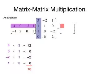
Matrix – matrix multiplication: C = A * B • C(:, :) = 0; for i = 1:n for j = 1:n for k = 1:n C(i, j) = C(i, j) + A(i, k) * B(k, j); • The n^3 scalar updates can be done in any order. • Six possible algorithms: ijk, ikj, jik, jki, kij, kji (lots more if you think about blocking for cache)
Organizations of matrix multiplication • How to do it in O(flops) time? • - How insert updates fast enough? • - How avoid (n2) loop iterations? • Loop k only over nonzeros in column j of B • Sparse accumulator • outer product: for k = 1:n C = C + A(:, k) * B(k, :) • inner product: for i = 1:n for j = 1:n C(i, j) = A(i, :) * B(:, j) • column by column: for j = 1:n for k = 1:n C(:, j) = C(:, j) + A(:, k) * B(k, j)
Sparse matrix data structures (one example) • Full: • 2-dimensional array of real or complex numbers • (nrows*ncols) memory • Sparse: • compressed column storage (CSC) • about (1.5*nzs + .5*ncols) memory
Sparse accumulator (SPA) • Abstract data type for a single sparse matrix column • Operations: • initialize spa O(n) time & O(n) space • spa = spa + (scalar) * (CSC vector) O(nnz(spa)) time • (CSC vector) = spa O(nnz(spa)) time (***) • spa = 0 O(nnz(spa)) time • … possibly other ops
Sparse accumulator (SPA) • Abstract data type for a single sparse matrix column • Operations: • initialize spa O(n) time & O(n) space • spa = spa + (scalar) * (CSC vector) O(nnz(spa)) time • (CSC vector) = spa O(nnz(spa)) time (***) • spa = 0 O(nnz(spa)) time • … possibly other ops • Implementation: • dense n-element floating-point array “value” • dense n-element boolean (***) array “is-nonzero” • linked structure to sequence through nonzeros (***) • (***) many possible variations in details
n1/2 The (2-dimensional) model problem • Graph is a regular square grid with n = k^2 vertices. • Corresponds to matrix for regular 2D finite difference mesh. • Gives good intuition for behavior of sparse matrix algorithms on many 2-dimensional physical problems. • There’s also a 3-dimensional model problem.
Permutations of the 2-D model problem • Theorem:With the natural permutation, the n-vertex model problem has (n3/2) fill. • Theorem:With any permutation, the n-vertex model problem has (n log n) fill. • Theorem:With a nested dissection permutation, the n-vertex model problem has O(n log n) fill.
Nested dissection ordering • Aseparatorin a graph G is a set S of vertices whose removal leaves at least two connected components. • A nested dissection ordering for an n-vertex graph G numbers its vertices from 1 to n as follows: • Find a separator S, whose removal leaves connected components T1, T2, …, Tk • Number the vertices of S from n-|S|+1 to n. • Recursively, number the vertices of each component:T1 from 1 to |T1|, T2 from |T1|+1 to |T1|+|T2|, etc. • If a component is small enough, number it arbitrarily. • It all boils down to finding good separators!
Separators in theory • If G is a planar graph with n vertices, there exists a set of at most sqrt(6n) vertices whose removal leaves no connected component with more than 2n/3 vertices. (“Planar graphs have sqrt(n)-separators.”) • “Well-shaped” finite element meshes in 3 dimensions have n2/3 - separators. • Also some other classes of graphs – trees, graphs of bounded genus, chordal graphs, bounded-excluded-minor graphs, … • Mostly these theorems come with efficient algorithms, but they aren’t used much.
Separators in practice • Graph partitioning heuristics have been an active research area for many years, often motivated by partitioning for parallel computation. See CS 240A. • Some techniques: • Spectral partitioning (uses eigenvectors of Laplacian matrix of graph) • Geometric partitioning (for meshes with specified vertex coordinates) • Iterative-swapping (Kernighan-Lin, Fiduccia-Matheysses) • Breadth-first search (GLN 7.3.3, fast but dated) • Many popular modern codes (e.g. Metis, Chaco) use multilevel iterative swapping • Matlab graph partitioning toolbox: see course web page
Heuristic fill-reducing matrix permutations • Nested dissection: • Find a separator, number it last, proceed recursively • Theory: approx optimal separators => approx optimal fill and flop count • Practice: often wins for very large problems • Minimum degree: • Eliminate row/col with fewest nzs, add fill, repeat • Hard to implement efficiently – current champion is “Approximate Minimum Degree” [Amestoy, Davis, Duff] • Theory: can be suboptimal even on 2D model problem • Practice: often wins for medium-sized problems • Banded orderings (Reverse Cuthill-McKee, Sloan, . . .): • Try to keep all nonzeros close to the diagonal • Theory, practice: often wins for “long, thin” problems • The best modern general-purpose orderings are ND/MD hybrids.
n1/2 n1/3 Complexity of direct methods Time and space to solve any problem on any well-shaped finite element mesh
Fill-reducing permutations in Matlab • Symmetric approximate minimum degree: • p = symamd(A); • symmetric permutation: chol(A(p,p)) often sparser than chol(A) • Symmetric nested dissection: • not built into Matlab • several versions in meshpart toolbox (course web page references) • Nonsymmetric approximate minimum degree: • p = colamd(A); • column permutation: lu(A(:,p)) often sparser than lu(A) • also for QR factorization • Reverse Cuthill-McKee • p = symrcm(A); • A(p,p) often has smaller bandwidth than A • similar to Sparspak RCM