Download

1 / 31
310 likes | 413 Views
Global Clustering Tests. Tests for Spatial Randomness. H 0 : The risk of disease is the same everywhere after adjustment for age, gender and/or other covariates. Tests for Global Clustering. Evaluates whether clustering exist as a global phenomena throughout the map, without

E N D
Tests for Spatial Randomness H0: The risk of disease is the same everywhere after adjustment for age, gender and/or other covariates.
Tests for Global Clustering Evaluates whether clustering exist as a global phenomena throughout the map, without pinpointing the location of specific clusters.
Tests for Global Clustering More than 100 different tests for global clustering proposed by different scientists in different fields. For example: • Whittemore’s Test, Biometrika 1987 • Cuzick-Edwards k-NN, JRSS 1990 • Besag-Newell’s R, JRSS 1991 • Tango’s Excess Events Test, StatMed 1995 • Swartz Entropy Test, Health and Place 1998 • Tango’s Max Excess Events Test, StatMed 2000
Cuzick-Edward’s k-NN Test åici åjcj I(dij<dik(i)) where ci = number of deaths in county i dij = distance from county i to county j k(i) = the county with the ‘k-nearest neighbor’ to an individual in county i, defined in terms of expected cases rather than individuals.
Cuzick-Edward’s k-NN Test Special case of the Weighted Moran’s I Test, proposed by Cliff and Ord, 1981
Tango’s Excess Events Test åi åj [cj-E(cj)] [cj-E(cj)] e-4d2ij/l2 where ci = number of deaths in county i E(cj) = expected cases in county i | H0 dij = distance from county i to county j l = clustering scale parameter
Whittemore's Test Whittemore et al. proposed the statistic
Besag- Newell’s R • For each case, find the collection of nearest counties so that there are a total of at least k cases in the area of the original and neighboring counties. • Using the Poisson distribution, check if this area is statistically significant (not adjusting for multiple testing) • R is the the number of cases for which this procedure creates a significant area
Besag-Newell's R Let um(i)=min{j:(Dj(i)+1) k}. Under null hypothesis, the case number s will have Poisson distribution with probability where p=C/N. For each county R is defined as
Swartz’s Entropy Test The test statistic is defined as where ni is the population in county I, and N is the total population
Global Clustering TestsPower Evaluation Joint work with Toshiro Tango, Peter Park and Changhong Song
Power Evaluation, Setup • 245 counties and county equivalents in Northeastern United States • Female population • 600 randomly distributed cases, according to different probability models
Note Besag-Newell’s R and Cuzick-Edwards k-NN tests depend on a clustering scale parameter. For each test we evaluate three different parameters.
Global Chain Clustering • Each county has the same expected number of cases under the null and alternative hypotheses • 300 cases are distributed according to complete spatial randomness • Each of these have a twin case, located at the same or a nearby location.
PowerZero Distance Besag-Newell 0.48 0.49 0.42 Cuzick-Edwards 1.00 0.92 0.73 Tango’s MEET 0.99 Swartz Entropy 1.00 Whittemore’s Test 0.13 Spatial Scan 0.79
PowerFixed Distance, 1% Besag-Newell 0.06 0.08 0.23 Cuzick-Edwards 0.16 0.32 0.38 Tango’s MEET 0.41 Swartz Entropy 0.14 Whittemore’s Test 0.12 Spatial Scan 0.28
PowerFixed Distance, 4% Besag-Newell 0.06 0.06 0.12 Cuzick-Edwards 0.06 0.06 0.07 Tango’s MEET 0.17 Swartz Entropy 0.06 Whittemore’s Test 0.10 Spatial Scan 0.12
PowerRandom Distance, 1% Besag-Newell 0.14 0.21 0.27 Cuzick-Edwards 0.53 0.52 0.47 Tango’s MEET 0.56 Swartz Entropy 0.39 Whittemore’s Test 0.12 Spatial Scan 0.35
PowerRandom Distance, 4% Besag-Newell 0.08 0.10 0.12 Cuzick-Edwards 0.14 0.17 0.18 Tango’s MEET 0.25 Swartz Entropy 0.13 Whittemore’s Test 0.10 Spatial Scan 0.18
Hot Spot Clusters • One or more neighboring counties have higher risk that outside. • Constant risks among counties in the cluster, as well as among those outside the cluster
PowerGrand Isle, Vermont (RR=193) Besag-Newell 0.71 0.39 0.09 Cuzick-Edwards 0.75 0.17 0.04 Tango’s MEET 0.20 Swartz Entropy 0.94 Whittemore’s Test 0.02 Spatial Scan 1.00
PowerGrand Isle +15 neigbors (RR=3.9) Besag-Newell 0.82 0.88 0.50 Cuzick-Edwards 0.76 0.62 0.25 Tango’s MEET 0.23 Swartz Entropy 0.71 Whittemore’s Test 0.01 Spatial Scan 0.97
PowerPittsburgh, PA (RR=2.85) Besag-Newell 0.04 0.02 0.98 Cuzick-Edwards 0.65 0.92 0.90 Tango’s MEET 0.92 Swartz Entropy 0.27 Whittemore’s Test 0.00 Spatial Scan 0.94
PowerPittsburgh + 15 neighbors (RR=2.1) Besag-Newell 0.29 0.28 0.91 Cuzick-Edwards 0.60 0.72 0.84 Tango’s MEET 0.83 Swartz Entropy 0.35 Whittemore’s Test 0.00 Spatial Scan 0.95
PowerManhattan (RR=2.73) Besag-Newell 0.04 0.03 0.95 Cuzick-Edwards 0.63 0.86 0.89 Tango’s MEET 0.94 Swartz Entropy 0.26 Whittemore’s Test 0.27 Spatial Scan 0.92
PowerManhattan + 15 neighbors (RR=1.53) Besag-Newell 0.01 0.06 0.37 Cuzick-Edwards 0.26 0.65 0.80 Tango’s MEET 0.99 Swartz Entropy 0.05 Whittemore’s Test 0.87 Spatial Scan 0.93
Power, Three ClustersGrand Isle (RR=193), Pittsburgh (RR=2.85), Manhattan (RR=2.73 Besag-Newell 0.54 0.18 1.00 Cuzick-Edwards 0.99 1.00 0.99 Tango’s MEET 1.00 Swartz Entropy 0.99 Whittemore’s Test 0.01 Spatial Scan 1.00
Power, Three ClustersGrand Isle +15, Pittsburgh +15, Manhattan +15 Besag-Newell 0.64 0.77 0.84 Cuzick-Edwards 0.91 0.96 0.96 Tango’s MEET 0.98 Swartz Entropy 0.74 Whittemore’s Test 0.12 Spatial Scan 0.98
Conclusions • Besag-Newell’s R and Cuzick-Edward’s k-NN often perform very well, but are highly dependent on the chosen parameter • Moran’s I and Whittemore’s Test have problems with many types of clustering • Tango’s MEET perform well for global clustering • The spatial scan statistic perform well for hot-spot clusters
Limitations • Only a few alternative models evaluated, on one particular geographical data set. • Results may be different for other types of alternative models and data sets.