Download

1 / 61
610 likes | 669 Views
The Power of Regression. Previous Research Literature Claim Foreign-owned manufacturing plants have greater levels of strike activity than domestic plants In Canada, strike rates of 25.5% versus 20.3% Budd’s Claim Foreign-owned plants are larger and located in strike-prone industries

E N D
The Power of Regression • Previous Research Literature Claim • Foreign-owned manufacturing plants have greater levels of strike activity than domestic plants • In Canada, strike rates of 25.5% versus 20.3% • Budd’s Claim • Foreign-owned plants are larger and located in strike-prone industries • Need multivariate regression analysis!
Important Regression Topics • Prediction • Various confidence and prediction intervals • Diagnostics • Are assumptions for estimation & testing fulfilled? • Specifications • Quadratic terms? Logarithmic dep. vars.? • Additional hypothesis tests • Partial F tests • Dummy dependent variables • Probit and logit models
Confidence Intervals • The true population [whatever] is within the following interval (1-)% of the time: Estimate ± t/2 Standard ErrorEstimate • Just need • Estimate • Standard Error • Shape / Distribution (including degrees of freedom)
Prediction Interval for New Observation at xp 1. Point Estimate 2. Standard Error 3. Shape • t distribution with n-k-1 d.f 4. So prediction interval for a new observation is 4. So prediction interval for a new observation is Siegel, p. 481
Prediction Interval for Mean Observations at xp 1. Point Estimate 2. Standard Error 3. Shape • t distribution with n-k-1 d.f 4. So prediction interval for a new observation is Siegel, p. 483
Earlier Example Hours of Study (x) and Exam Score (y) Example • Find 95% CI for Joe’s exam score (studies for 20 hours) • Find 95% CI for mean score for those who studied for 20 hours - x = 18.80
Diagnostics / Misspecification • For estimation & testing to be valid… • y = b0 + b1x1 + b2x2 + … + bkxk + e makes sense • Errors (ei) are independent • of each other • of the independent variables • Homoskedasticity • Error variance independent of the independent variables • e2 is a constant • Var(ei) xi2 (i.e., not heteroskedasticity) Violations render our inferences invalid and misleading!
Common Problems • Misspecification • Omitted variable bias • Nonlinear rather than linear relationship • Levels, logs, or percent changes? • Data Problems • Skewed variables and outliers • Multicollinearity • Sample selection (non-random data) • Missing data • Problems with residuals (error terms) • Non-independent errors • Heteroskedasticity
Omitted Variable Bias • Question 3 from Sample Exam B wage = 9.05 + 1.39 union (1.65) (0.66) wage = 9.56 + 1.42 union + 3.87 ability (1.49) (0.56) (1.56) wage = -3.03 + 0.60 union + 0.25 revenue (0.70) (0.45) (0.08) • H. Farber thinks the average union wage is different from average nonunion wage because unionized employers are more selective and hire individuals with higher ability. • M. Friedman thinks the average union wage is different from the average nonunion wage because unionized employers have different levels of revenue per employee.
Checking the Assumptions • How to check the validity of the assumptions? • Cynicism, Realism, and Theory • Robustness Checks • Check different specifications • But don’t just choose the best one! • Automated Variable Selection Methods • e.g., Stepwise regression (Siegel, p. 547) • Misspecification and Other Tests • Examine Diagnostic Plots
Diagnostic Plots Increasing spread might indicate heteroskedasticity. Try transformations or weighted least squares.
Diagnostic Plots “Tilt” from outliers might indicate skewness. Try log transformation
Problematic Outliers Stock Performance and CEO Golf Handicaps (New York Times, 5-31-98) Number of obs = 44 R-squared = 0.1718 ------------------------------------------------ stockrating | Coef. Std. Err. t P>|t| -------------+---------------------------------- handicap | -1.711 .580 -2.95 0.005 _cons | 73.234 8.992 8.14 0.000 ------------------------------------------------ Without 7 “Outliers” Number of obs = 51 R-squared = 0.0017 ------------------------------------------------ stockrating | Coef. Std. Err. t P>|t| -------------+---------------------------------- handicap | -.173 .593 -0.29 0.771 _cons | 55.137 9.790 5.63 0.000 ------------------------------------------------ With the 7 “Outliers”
Are They Really Outliers?? Diagnostic Plot is OK BE CAREFUL! Stock Performance and CEO Golf Handicaps (New York Times, 5-31-98)
Diagnostic Plots Curvature might indicate nonlinearity. Try quadratic specification
Diagnostic Plots Good diagnostic plot. Lacks obvious indications of other problems.
Adding Squared (Quadratic) Term Job Performance regression on Salary (in $1,000s) (Egg Data) Source | SS df MS Number of obs = 576 ------- -+-------------------- F(2,573) = 122.42 Model | 255.61 2 127.8 Prob > F = 0.0000 Residual | 598.22 573 1.044 R-squared = 0.2994 ---------+-------------------- Adj R-squared = 0.2969 Total | 853.83 575 1.485 Root MSE = 1.0218 ---------------+-------------------------------------------- job performance| Coef. Std. Err. t P>|t| ---------------+-------------------------------------------- salary | .0980844 .0260215 3.77 0.000 salary squared | -.000337 .0001905 -1.77 0.077 _cons | -1.720966 .8720358 -1.97 0.049 ------------------------------------------------------------ Salary Squared = Salary2 [=salary^2 in Excel]
Quadratic Regression Job perf = -1.72 + 0.098 salary – 0.00034 salary squared Quadratic regression (nonlinear)
-linear coeff. Max = 2*quadratic coeff. Quadratic Regression Job perf = -1.72 + 0.098 salary – 0.00034 salary squared Effect of salary will eventually turn negative But where?
Another Specification Possibility • If data are very skewed, can try a log specification • Can use logs instead of levels for independent and/or dependent variables • Note that the interpretation of the coefficients will change • Re-familiarize yourself with Siegel, pp. 68-69
Quick Note on Logs • a is the natural logarithm of x if: 2.71828a = x or, ea = x • The natural logarithm is abbreviated “ln” • ln(x) = a • In Excel, use ln function • We call this the “log” but don’t use the “log” function! • Usefulness: spreads out small values and narrows large values which can reduce skewness
Earnings Distribution Skewed to the right Weekly Earnings from the March 2002 CPS, n=15,000
Residuals from Levels Regression Skewed to the right—use of t distribution is suspect Residuals from a regression of Weekly Earnings on demographic characteristics
Log Earnings Distribution Not perfectly symmetrical, but better Natural Logarithm of Weekly Earnings from the March 2002 CPS, i.e., =ln(weekly earnings)
Residuals from Log Regression Almost symmetrical—use of t distribution is probably OK Residuals from a regression of Log Weekly Earnings on demographic characteristics
Hypothesis Tests • We’ve been doing hypothesis tests for single coefficients • H0: = 0 reject if |t| > t/2,n-k-1 • HA: 0 • What about testing more than one coefficient at the same time? • e.g., want to see if an entire group of 10 dummy variables for 10 industries should be in the model • Joint tests can be conducted using partial F tests
Partial F Tests H0: 1 = 2 = 3 = … = C = 0 HA: at least one i 0 • How to test this? • Consider two regressions • One as if H0 is true • i.e., 1 = 2 = 3 = … = C = 0 • This is a “restricted” (or constrained) model • Plus a “full” (or unconstrained) model in which the computer can estimate what it wants for each coefficient
Partial F Tests • Statistically, need to distinguish between • Full regression “no better” than the restricted regression – versus – • Full regression is “significantly better” than the restricted regression • To do this, look at variance of prediction errors • If this declines significantly, then reject H0 • From ANOVA, we know ratio of two variances has an F distribution • So use F test
Partial F Tests • SSresidual = Sum of Squares Residual • C = #constraints • The partial F statistic has C, n-k-1 degrees of freedom • Reject H0 if F > F,C, n-k-1
Minitab Output Predictor Coef StDev T P Constant -168.5 258.8 -0.65 0.519 hours 1.2235 0.186 6.56 0.000 tons 0.0478 0.403 0.12 0.906 unemp 19.618 5.660 3.47 0.001 WWII 159.85 78.22 2.04 0.048 Act1952 -9.8 100.0 -0.10 0.922 Act1969 -203.0 111.5 -1.82 0.076 S = 108.1 R-Sq = 95.5% R-Sq(adj) = 94.9% Analysis of Variance Source DF SS MS F P Regression 6 9975695 1662616 142.41 0.000 Error 40 467008 11675 Total 46 10442703
Is the Overall Model Significant? H0: 1 = 2 = 3 = … = 6 = 0 HA: at least one i 0 • Note: for testing the overall model, C=k • i.e., testing all coefficients together • From the previous slides, we have SSresidual for the “full” (or unconstrained) model • SSresidual=467,007.875 • But what about for the restricted (H0 true) regression? • Estimate a constant only regression
Partial F Tests = 142.406 H0: 1 = 2 = 3 = … = 6 = 0 HA: at least one i 0 • Reject H0 if F > F,C, n-k-1 = F0.05,6,40 = 2.34 • 142.406 > 2.34 so reject H0. Yes, overall model is significant
Select F Distribution 5% Critical Values Denominator Degrees of Freedom
A Small Shortcut For constant only model, SSresidual=10,442,702.809 So to test overall model, you don’t need to run a constant-only model
An Even Better Shortcut In fact, the ANOVA table F test is exactly the test for the overall model being significant—recall Unit 8
Testing Any Subset Partial F test can be used to test any subset of variables For example, H0: WWII = Act1952 = Act1969 = 0 HA: at least one i 0
Restricted Model Restricted regression with WWII = Act1952 = Act1969 = 0
Partial F Tests = 3.950 H0: WWII = Act1952 = Act1969 = 0 HA: at least one i 0 • Reject H0 if F > F,C, n-k-1 = F0.05,3,40 = 2.84 • 3.95 > 2.84 so reject H0. Yes, subset of three coefficients are jointly significant
Regression and Two-Way ANOVA Blocks “Stack” data using dummy variables
Regression and Two-Way ANOVA Source | SS df MS Number of obs = 15 ----------+---------------------- F( 6, 8) = 28.00 Model | 338.800 6 56.467 Prob > F = 0.0001 Residual | 16.133 8 2.017 R-squared = 0.9545 -------------+------------------- Adj R-squared = 0.9205 Total | 354.933 14 25.352 Root MSE = 1.4201 ------------------------------------------------------------- treatment | Coef. Std. Err. t P>|t| [95% Conf. Int] ----------+-------------------------------------------------- b | -2.600 .898 -2.89 0.020 -4.671 -.529 c | -3.000 .898 -3.34 0.010 -5.071 -.929 b2 | -1.333 1.160 -1.15 0.283 -4.007 1.340 b3 | 6.667 1.160 5.75 0.000 3.993 9.340 b4 | 9.667 1.160 8.34 0.000 6.993 12.340 b5 | -1.333 1.160 -1.15 0.283 -4.007 1.340 _cons | 10.867 .970 11.20 0.000 8.630 13.104 -------------------------------------------------------------
Regression and Two-Way ANOVA Regression Excerpt for Full Model Source | SS df MS ---------+------------------- Model | 338.800 6 56.467 Residual | 16.133 8 2.017 ---------+------------------- Total | 354.933 14 25.352 Use these SSresidual values to do partial F tests and you will get exactly the same answers as the Two-Way ANOVA tests Regression Excerpt for b2= b3 =… 0 Source | SS df MS ---------+------------------- Model | 26.533 2 13.267 Residual | 328.40 12 27.367 ---------+------------------- Total | 354.933 14 25.352 Regression Excerpt for b= c = 0 Source | SS df MS ---------+------------------- Model | 312.267 4 78.067 Residual | 42.667 10 4.267 ---------+------------------- Total | 354.933 14 25.352
Select F Distribution 5% Critical Values Denominator Degrees of Freedom
Regression Coefficients • y = b0 + b1x (linear form) • log(y) = b0 + b1x (semi-log form) • log(y) = b0 + b1log(x) (double-log form) 1 unit change in x changes y by b1 1 unit change in x changes y by b1 (x100)percent 1 percent change in x changes y by b1 percent
Log Regression Coefficients • wage = 9.05 + 1.39 union • Predicted wage is $1.39 higher for unionized workers (on average) • log(wage) = 2.20 + 0.15 union • Semi-elasticity • Predicted wage is approximately 15% higher for unionized workers (on average) • log(wage) = 1.61 + 0.30 log(profits) • Elasticity • A one percent increase in profits increases predicted wages by approximately 0.3 percent
Multicollinearity Auto repair records, weight, and engine size Number of obs = 69 F( 2, 66) = 6.84 Prob > F = 0.0020 R-squared = 0.1718 Adj R-squared = 0.1467 Root MSE = .91445 ---------------------------------------------- repair | Coef. Std. Err. t P>|t| -------+-------------------------------------- weight | -.00017 .00038 -0.41 0.685 engine | -.00313 .00328 -0.96 0.342 _cons | 4.50161 .61987 7.26 0.000 ----------------------------------------------