Electron Probe Microanalysis EPMA

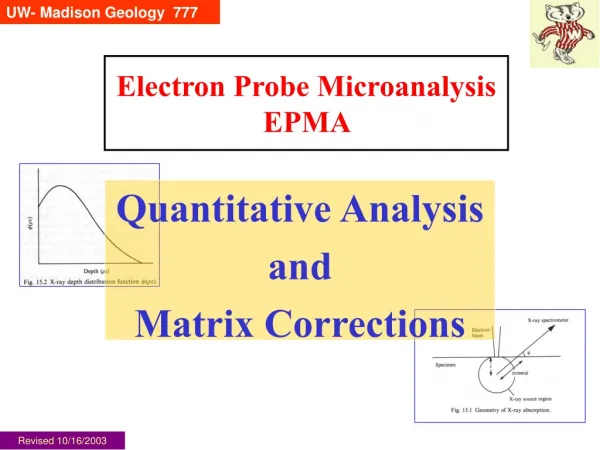
UW- Madison Geology 777 Electron Probe MicroanalysisEPMA Quantitative Analysis and Matrix Corrections Revised 10/29/2009

UW- Madison Geology 777 K ratios Recall Castaing’s approach to quantitative analysis, where specimen intensities are ratioed to standard intensities: where K is the “K ratio” for element i, I is the X-ray intensity of the phase and subscript i is the element. With the counts acquired on BOTH unknowns and standards on the same instrument, under the same operating conditions, we assume that many physical parameters of the machine that would be needed in a rigorous physical model cancel each other out (same in numerator and denominator).

UW- Madison Geology 777 Castaing’s First Approximation Castaing’s “first approximation” follows this approach. The composition C of element i of the unknown is the K ratio times the composition of the standard. In the simple case where the standard is the pure element, then, the fraction K is roughly equal to the fraction of the element in the unknown.

UW- Madison Geology 777 ...close but not exact However, it was immediately obvious to Castaing that the raw data had to be corrected in order to achieve the full potential of this new approach to quantitative microanalysis. The next two slides give a graphic demonstration of the need for development of a correction procedure.

UW- Madison Geology 777 This plot of Fe Ka X-ray intensity data demonstrates why we must correct for matrix effects. Here 3 Fe alloys show distinct variations. Consider the 3 alloys at 40% Fe. X-ray intensity of the Fe-Ni alloy is ~5% higher than for the Fe-Mn, and the Fe-Cr is ~5% lower than the Fe-Mn. Thus, we cannot use the raw X-ray intensity to determine the compositions of the Fe-Ni and Fe-Cr alloys. Raw data needs correction (Note the hyperbolic functionality of the upper and lower curves)

UW- Madison Geology 777 Absorption and Fluorescence • Note that the Fe-Mn alloys plot along a 1:1 line, and so is a good reference. • The Fe-Ni alloys plot above the 1:1 line (have apparently higher Fe than they really do), because the Ni atoms present produce X-rays of 7.278 keV, which is greater than the Fe K edge of 7.111 keV.Thus, additional Fe Ka are produced by this secondary fluorescence. • The Fe-Cr alloys plot below the 1:1 line (have apparently lower Fe than they really do), because the Fe atoms present produce X-rays of 6.404 keV, which is greater than the Cr K edge of 5.989 keV. Thus, Cr Ka is increased, with Fe Ka are “used up” in this secondary fluorescence process.

UW- Madison Geology 777 Two approaches to corrections • In his 1951 Ph.D. thesis, Castaing laid out the two approaches that could be used to apply matrix corrections to the data: • an empirical ‘alpha factor’ correction for binary compounds, where each pair of elements has a pair of constant a-factors representing the effect that each element has upon the other for measured X-ray intensity, and • a more rigorous physical model taking into account absorption and fluorescence in the specimen. This later approach also includes atomic number effects and became known as ZAF correction.

UW- Madison Geology 777 Z A F In addition to absorption (A) and fluorescence (F), there are two other matrix corrections based upon the atomic number (Z) of the material: one dealing with electron backscattering, the other with electron penetration (or stopping). These deal with corrections to the generation of X-rays.C is composition as wt% element (or elemental fraction). We will now go through all these corrections in some detail, starting with the Z correction, which has two parts, the stopping power correction, and the backscatter correction. Note that all these corrections require close attention to exactly what feature’s value is being input: the target (matrix), or the X-ray in question.

UW- Madison Geology 777 Stopping Power Correction Incident electrons lose energy in inelastic interactions with the inner shell electrons of the target. The “stopping power” (energy lost by HV electrons per unit mass penetrated) is not constant but drops with increasing Z. A higher number of X-rays will be produced in higher Z targets. Thus, if the mean Z of the unknown is higher than that of the standard, a downward correction in the composition must be applied. The stopping power correction factor is “S”, and can be approximated by: Reed, 1996, Fig. 8.6, p. 135 Stopping power of pure elements for 20 keV electrons where J=11.5+ Z and Emean= (E0+Ec)/2 (J is the mean ionization energy; J, Z and A are of the target, Emean is of the X-ray)

UW- Madison Geology 777 Backscatter Correction Reed, 1996, Fig. 2.11, p. 17 As we discussed earlier, the fraction of high energy incident elections that are backscattered (h) increases with atomic number. There then will be relatively less incident electrons penetrating into higher Z specimens, resulting in a smaller number of X-rays. Thus, if the mean Z of the unknown is higher than that of the standard, a upward correction in the composition must be applied. The backscatter correction factor is “R”. R can be approximated by where W = Ec/E0 (the inverse of overvoltage), and Z is of the target, and W is of the X-ray

UW- Madison Geology 777 Z correction The total atomic number correction is formed by multiplication of the R and S of the unknown and standard thusly: Z = Rstd/Runk * Sunk/Sstd Overall the backscatter and the stopping power corrections tend to cancel each other out.But if there is a (small) correction, it is usually in the direction of the backscatter correction.

UW- Madison Geology 777 Beers Law The intensity I of X-rays that pass through a substance are subject to attenuation of their initial intensity I0 by the material over the distance they travel within the material. The attenuation follows an exponential decay with a characteristic linear attenuation length 1/m, where m is the (linear) absorption coefficient. Beers Law can also be expressed in terms of mass, using density terms: I = I0 exp -(m/r)(r Z) where (m/r) is the mass absorption coefficient (cm2/g), r is the material density (g/cm3), and Z is the distance (cm) Als-Nielsen and McMorrow, 2001, Fig 1.10, p. 19

UW- Madison Geology 777 Mass Absorption Coefficients Mass absorption coefficients (MACs) have been tabulated* for many X-rays through many substances (though some are extrapolations). They exist as a matrix of numbers: absorption of a particular X-ray line (emitter, e.g. Ga ka) by a absorber or target (e.g. As) will have one value (51.5). Note that the absorption of As Ka by Ga is a totally different phenomenon with a distinct MAC (221.4) . Emitter = X-ray (here, Ka) Absorber = matrix material *See following discussion Goldstein et al, 1992, p. 750.

UW- Madison Geology 777 Mass Absorption Coefficients Emitter = X-ray (here, Ka) Terminology: “the mass absorption of Ga Kaby As” Question for you: Is the mass absorption of As Ka by Ga the same as the mass absorption of Ga Ka by As? Why or why not? Absorber = matrix material Goldstein et al, 1992, p. 750.

UW- Madison Geology 777 X-rays produced within the material will be propagated in all directions, and will suffer attenuation in the process. Note that the path length of travel of the X-ray to the spectrometer is z cosecy, where y (psi) is the takeoff angle (cosec = 1/sin). Castaing’s approach was to integrate the Beer’s Law equation over the depth at the given y, producing the absorption correction factor f(c) where c is defined as m cosec y where m is the MAC. The absorption (A) correction is then defined as A= f(c)std / f(c)sample Absorption Reed, 1993,, p. 219

UW- Madison Geology 777 Absorption To be able to correct for this absorption of the measured X-rays, we need to know how the production of X-rays varies with depth (Z) in the material. The distribution of X-rays as a function of depth is known as the f(rz) [phi-rho-z] function, where a “mass depth” parameter is used instead of simple z (bottom right). The f(rz) function is defined as the intensity generated in a thin layer at some depth z, relative to that generated in an isolated layer of the same thickness. Reed, 1993, p. 219

UW- Madison Geology 777 Absorption One commonly used simplified form (Philibert 1963) is where c = m cosec y , s is a measure of electron absorption and depends on effective electron energy, where The Philibert approximation breaks down, however, at the near surface, creating errors when dealing with low energy light elements, and we need to go to more complicated and accurate forms of the f(rz) function. Reed, 1993, p. 219

UW- Madison Geology 777 f(rz) [phi-rho-z] Curves To be able to correct properly for absorption -- particularly for light elements, the exact shape of the f(rz) [phi-rho-z] curve must be known. Each X-ray has its own curve. There are 3 main parameters that affect the shape of the curve: • E0 (accelerating voltage) • Ec (critical excitation energy of a particular element line • mean Z of the material Reed, 1993, p. 220

UW- Madison Geology 777 Tracer Method The f(rz) [phi-rho-z] curves are usually determined by the “tracer method”, where successive layers are deposited by vacuum evaporation. The tracer layer B is deposited atop substrate A, with successive layers of A deposited on top. Characteristic X-rays from the tracer element are measured (“emitted”) and then a generation curve is calculated by correcting each step for absorption and fluorescence effects

UW- Madison Geology 777 Fluorescence Correction The X-rays produced within a specimen have the potential for producing a second generation of X-rays: this is secondary fluorescence, generally shortened to fluorescence. This occurs when the characteristic X-ray has an energy greater than the absorption edge energy of another element present in the specimen. As we saw earlier, Ni Ka (7.48 keV) is able to fluoresce Fe Ka (Ec 7.11 keV). This effect is maximized when there is a small amount of the fluoresced element present, e.g. Fe in a Ni-Fe alloy. Reed gives an example where the Fe intensity is 142% of what it “should be”. Also, the continuum above an absorption edge also causes fluorescence, although this is generally weak. Reed, 1996, Fig. 8.10, p. 139

UW- Madison Geology 777 Fluorescence Correction The form of the correction F is where If/Ip is the ratio of emitted X-rays from fluorescence, compared to the X-ray intensity from inner shell ionization. In a compound, this term is summed overall all the elements that could fluorescence the element of interest.

UW- Madison Geology 777 Secondary fluorescence is an important issue that must be appreciated. Generated X-rays are not scattered nearly as much as incident electrons, and thus the generated X-rays can travel relatively long distances (50 um in Fig 3.49) within the specimen and produce a second generation of X-rays. If the specimen (and standards) are relatively large (=homogeneous), this is not a problem. However, if minor or trace elements are being analyzed in small grains (Phase 1 in Fig 16.10) and the host phase (2) has high abundance, an error may be made in the EPMA analysis. Fluorescence Problems Goldstein et al. p. 142; Reed 1993, p. 258

UW- Madison Geology 777 Cu Co Secondary fluorescence is a potential source of analytical error across linear boundaries, either horizontal (e.g. thin films) or vertical (e.g., diffusion couples). In the example here of a vertical interface between untreated Cu and Co, there is NO diffusion. However, the resulting EPMA profiles clearly imply there is diffusion. There is NO diffusion – there is only secondary fluorescence across the boundary. Cu Ka X-rays can excite Co, to the extent that there is apparently 1 wt% Co about 15 um away from the boundary within the Cu. But Co Ka cannot excite Cu, so only the continuum X-rays can create secondary fluorescence, which is less – but certainly distinguishable, an apparent 0.5 wt% Cu at 10 um from the boundary in the Co. Fluorescence across boundaries Reed 1993, p. 259-260 “false Co” “false Cu”

UW- Madison Geology 777 Another lab reported 10 wt% Nb (below) in what should have been Nb-free phase (by EDS at 30 kV). The issue was small grain size and nearby Nb (right image) An SF real story When I ran WDS (18 kV) I found essentially zero Nb -- what is the problem? The original researchers used Nb Ka because, with EDS, it is impossible to resolve Nb La (it sits between Al Ka, Hf Ma and Pd La). Above: EDS spectrum on Pd2HfAl 5 um away from Nb. Pd Ka is very efficient at traveling across the border and exciting the Nb Fournelle, Kim and Perepezko (2005)

UW- Madison Geology 777 A recent article (below left) reports an innovative approach to correcting the secondary fluorescence (SF) in diffusion couples and from adjacent phases. This utilizes a complex Monte Carlo program called PENELOPE (Penetration and Energy Loss of Positrons and Electrons) that permits complicated geometric models of electron and X-ray behavior in materials. SF can be simulated in a model that represents the actual specimen (e.g. Fig 1 below), and then subtracted from the observed data (right figure). Secondary Fluorescence Correction

UW- Madison Geology 777 • The raw X-ray intensities are first corrected for: • background contribution • beam drift (i.e. counts are normalized) • deadtime • interferences* (if appropriate) • and then the K-ratios are input into an automated matrix correction program. • To run, the correction calculations must assume an initial composition for the unknown -- because the magnitude of each factor is proportional to the abundance of the element times its correction in a pure end member. The assumed composition is a normalized (to 100%) value of the K-ratio. Based upon the first iteration with this assumed composition, the result gives a more truer composition, which then is the input for the second iteration. The process is iterated until convergence, usually 3-5 times. Matrix Correction Programs * Probe for Windows does the interference correction within the matrix correction, a far better approach compared to the normal (antiquainted) procedure of correcting the data after the matrix correction is completed.

UW- Madison Geology 777 One currently widely used matrix correction program is CITZAF, developed by John Armstrong (then CIT, now at American Univ.) and implemented in our Probe for Windows software. There are several options, which we elucidate here, but that generally we do not modify them from the default values. Probably the only parameter you would ever modify would be mass absorption coefficients (there are different ones for the light elements). ZAF options

UW- Madison Geology 777 Alpha correction In the early decades of probing when computer power was negligible, the alpha correction technique was widely used, as it required less number crunching and relied mainly on empirical data and less on complex physical models and physics. Today, however, there may be a rekindled interest in this approach, as it may “work better” in many cases.

Geology 777 Ziebold and Ogilvie - binary a-factors In 1963-4, Ziebold and Ogilvie* developed a corrections for some binary metal alloys, with an equation in the form where a12 is the a-factor for element 1 in the binary with element 2, K is the K-ratio, and composition (fractional) is C. This equation can be rearranged in the form If experimental data exist for binary alloys, then a plot of C1/K1 versus C1 is a straight line with a slope of (1- a12), leading to determination of a12. Such a hyperbolic relationship between C1 and K1 was shown to be correct for several alloy and oxide systems, but it was difficult to find appropriate intermediate compositions for many binary systems. = C2 = K2 *Quantitative Analysis with the Electron Microanalyzer, Analytical Chemistry, Vol 35, May 1963, p. 621-627; An Empirical Method for Electron Microanalysis, Analytical Chemistry, Vol 36, Feb. 1964, p. 322-327.

UW- Madison Geology 777 Ziebold and Ogilvie - ternary a-factors Ziebold and Ogilvie showed that a corrections could be developed for some ternary metal alloys, with an equation in the form where a123 is the a-factor for element 1 in the ternary with elements 2 and 3, and is defined as This equation can be rearranged Similar relationships can be written for elements 2 and 3, and used to calculate a-factors for the 3 binary systems of the ternary.These a-factors were limited to a particular E0 and takeoff angle.

UW- Madison Geology 777 Bence-Albee -multicomponent systems Bence and Albee* in 1968 showed that this approach could be extended to silicates and other minerals, i.e. a system of n components, where for the nth component a b-factor could be found where where an1 is the a-factor for the n1 binary. These factors were determined for a limited set of conditions, i.e. 15 and 20 keV, and take off angles of 52.5° and 38.5°. The 1968 Bence and Albee paper is one of the most highly cited papers in the geological literature (over ~20,000 citations). * Empirical correction factors for the electron microanalysis of silicates and oxides, J. Geology, Vol. 76, p. 382-403; also see Albee and Ray, Correction Factors for Electron Probe Microanalysis of Silicates, Oxides, Carbonates, Phosphates, and Sulfates, Analytical Chemistry, Vol 42, Oct 1970, p. 1408-1414.

UW- Madison Geology 777 In 1988, John Armstrong* reviewed the Bence-Albee (a-factor) correction scheme for EPMA of oxide and silicate minerals. He evaluated the old factors, and revised some, using a -factors calculated from newer ZAF and f(rz)algorithms, and showed “that with some modifications the a -factor corrections can be as accurate as any other correction procedure currently available and much easier and quicker to process.” Evaluating matrix corrections *Bence-Albee after 20 years: review of the accuracy of a-factor correction procedures for oxide and silicate minerals, in Microbeam Analysis-1988, p. 469-76. Armstrong also reviewed† ZAF and f(rz) corrections and suggested that some of these correction algorithms “produce poorer results in the analysis of silicate and oxide minerals than some of the earlier corrections”. He specifically was referring to various corrections that were optimized for metal alloys † Quantitative analysis of silicate and oxide materials: comparison of Monte Carlo, ZAF and f(rz) procedures, in Microbeam Analysis-1988, p. 239+

UW- Madison Geology 777 Unanalyzed elements The matrix corrections assume that all elements present (and interacting with the X-rays) will be included. There are situations, however, where either an element cannot be measured, or not easily, and thus the analyst must make explicit in the quantitative setup the presence of unanalyzed element/s -- and how they are to be input into the correction. Before we forget.... Typically oxygen (in silicates) is calculated “by stoichometry”. Elements can also be defined in set amounts, or relative proportions, or “by difference” – although this later method is somewhat dangerous as it assumes that there are no other elements present.

UW- Madison Geology 777 Unanalyzed oxygen, carbon, etc Oxygen is a major part of many materials (e.g. silicate minerals and glasses). Carbon is a major part of carbonates. Oxygen and carbon are typically not “acquired” (measured directly) in many EPMA procedures, BUT THEY MUST BE SOMEHOW INCLUDED IN THE MATRIX CORRECTION. If oxygen (and say C in carbonates) is not included, there will be errors in the matrix corrections of some elements, as the presence these elements affects the electron (and x-ray behavior), e.g., the backscattered % of incident HV electrons will be different, and there may be absorption of those x-rays by the oxygen (and C) present. In the next slides, we see the effect on a measurement of a carbonate sample: first, with just the cations; then with just Oxygen added; finally with both Oxygen and Carbon.

UW- Madison Geology 777 First: how you do it For a carbonate Declare C and O as elements in the analysis (but not measured) Tell it to calculate with stoichiometric oxygen Create a rule so that there is 1 atom of C to every 3 atoms of O Check: display results on basis of 3 atoms of oxygen (perfect result would be 5.000 total atoms, and grand total of 100 wt%

UW- Madison Geology 777 Good, Bad, Ugly …. Carbonate by EPMA First, if only cations used for ZAF … If both O and C included in the ZAF Next, oxygen only included … Notice the differences in the final values of the elements (wt%)

UW- Madison Geology 777 * Tingle, T.N., Neuhoff, P., Ostgergren, P., Jones, R.E. and Donovan, J.J. (1996) The effect of “missing” unanalyzed oxygen on quantitative electron probe microanalysis of hydrous silicate and oxide minerals. GSA Abstracts, 28, 212. Unanalyzed oxygen One complication for oxygen is variable valence states of elements such as Fe. Robust software will allow you to enter case by case different valence states. In some cases, if oxygen is not included, there can be errors in the matrix corrections of some elements, as the presence of O, OH, and H2O can affect the actually measured elements, as there may be significant absorption of those x-rays by the oxygen present*.

UW- Madison Geology 777 Consider: Apophyllite -- KCa4Si8O20(F,OH)•8 H2O Which has LOTS of oxygen which typically is “unanalyzed” and therefore not involved in the matrix correction Impact of unaccounted for oxygen Solution: Iterate a fixed amount of H2O (16 atoms of H = 1.76 wt% H plus stoichometric O) per formula to achieve good results. As shown in the bottom analysis where the H2O is missing, there is up to 3% relative error for cations.

UW- Madison Geology 777 Physical Parameters Needed The ZAF corrections require accurate and precise knowledge about many physical parameters, such as • Electron stopping power • Mean ionization potentials • Backscatter coefficients • X-ray Ionization cross sections • Mass absorption coefficients • Surface ionization potentials • Fluorescent yields

UW- Madison Geology 777 “State of EPMA parameters” • As David Joy points out in his 2001 article “Constants for Microanalysis”, there are problems in our knowledge of many parameters: • there are experimental stopping power profiles for 12 elements and 12 compounds, which raise questions about the traditional Bethe equation • only half of the elements whose K lines are used for EPMA have measured K shell ionization cross-sections ; only 6 elements have measured L shell cross-sections; there are zero M shell cross-sections • K shell fluorescent yields are the best documented parameters; there are gaps in the data for L shell yields; there are only 5 measured M shell yields • despite the fact that backscatter coefficients have been measured for 100 years, the data has many gaps and is of poor precision (i.e. 30%)

UW- Madison Geology 777 • At the Eugene EPMA workshop in September 2003, John Armstrong reviewed the state of EPMA matrix corrections • Big problem with software/manufacturers, not documenting which corrections used. Some have picked "improved" parameters which do not fit with the other parameters, e.g. in some, where no formal fluorescence correction, the absorption correction was tweaked to take fluor into account, and then when later fluorescence corrections developed, to use this in addition to absorption correction, has an overcorrection for fluorescence. • Problem with researchers not stating in their publications which correction they used; NIST is trying to develop some protocols which people can reference (brief notation with pointer to NIST for full description). • There are a few errors/typos in the long accepted X-ray tables (i.e., Bearden) – 3 are major errors. • Actually measured mass absorption factors are rare! Measurements exist for Na Ka by Al; Si Ka by Al and Ni; Mg Ka by O, Al, Ti and Ni; and Al Ka by O, Na ..... • There is over 30% variation in published values of some macs for geologically relevant elements; they can’t all be correct!

UW- Madison Geology 777 “So what do we do?” We have discussed various ways to correct the raw data, the goal being to come up with the most accurate and precise analytical procedures to give us the most trustworthy data. We have just mentioned that everything is not as rosy as one would hope. So, can we trust the numbers we get out of the probe? In many/most cases, given care, yes. But we cannot blindly look at the electron probe and computer as a black box! Stay tuned for an upcoming installment, where we discuss standards, accuracy and precision in EPMA.

Electron Probe Microanalysis EPMA