Download
1 / 31
310 likes | 444 Views
Daniele Montanino Università degli studi di Lecce and INFN. Neutrino decay and the supernova relic neutrino background. Based on: G.L. Fogli, E. Lisi, A. Mirizzi, D. M. Phys. Rev. D 70 013001 (2004) hep-ph/0401227. Introduction. We have now a striking evidence for neutrino oscillations

E N D
Daniele Montanino Università degli studi di Lecce and INFN Neutrino decay and the supernova relic neutrino background Based on: G.L. Fogli, E. Lisi, A. Mirizzi, D. M. Phys. Rev. D 70 013001 (2004) hep-ph/0401227
Introduction • We have now a striking evidence for neutrino oscillations • What about other non standard neutrino properties? • magnetic moment • VLI, VEP • non standard interactions • extra dimensions • quantum decoherence • sterile neutrinos • CPT violations • decay
Inverted Hierarchy (IH) Normal Hierarchy (NH) 2 3 m2 1 m2>0 m2 m2<0 2 m2 3 1 Framework • We stick in the current phenomenology of three generations of massive neutrinos. We do not consider: • heavy active neutrinos evading the LEP limit (m45GeV) • light or heavy sterile neutrinos • We also assume that mO(1eV) As of Neutrino’04 m28.210-5eV2 m22.410-3eV2 sin2120.28 sin213<0.07
Probing neutrino decay At the moment there are not experimental evidences in favour of decay. In order to leave “unperturbed” the current phenomenology, the decay lifetime should be sufficiently long. Roughly speaking, for a neutrino with mass m and energy E must be (in unit c=1): where is the proper (rest frame) neutrino lifetime, E/m is the Lorentz time-dilatation factor and L is the decay path length. For a given neutrino energy and decay path length a bound on /m can be fixed.
Types of neutrino decay For light neutrinos we have only two possible decays • “visible” (or “radiative”): • H L + • “invisible”: • H L + X or • H 3L • where “X” is massless (or a light) weak interacting particle (e.g., a Majoron)
The Majoron Model In some models of neutrino mass generation (see e.g., Gelmini & Roncadelli, Phys. Lett. B 99, 411, 1981), neutrinos are coupled with a massless Nambu-Goldstone boson, used called “Majoron” through a renormalizabe coupling: where the i,j are the Majorana neutrino mass eigenstates. If mj>mi the decays are possible.
Big Bang relic neutrinos cannot limit the neutrino-Majoron couplings. Indeed, in a recent work by Beacom et al. (astro-ph/0404585) has been shown that, within the current bounds on the couplings, almost all relic neutrinos annihilate each other through the reaction without affecting the current phenomenology (CMBR anisotropies, power spectrum). Neutrino decay into Majoron was also invoked by Barger et al. (Phys. Rev. Lett. 82, 2640, 1999) as an alternative explanation of the atmospheric neutrino anomaly. However, this model is now strongly disfavoured by the observation of a “dip” in the L/E distribution of events in SuperK.
m 1) “Strongly Hierarchical” (SH) case: mj>>mi j i 0 2) “Quasi Degenerate” (QD) case: mjmi (mij2=mj2-mi2) m j i 0 The intrinsic decay rate in vacuum has been calculated by Kim & Lam, Mod. Phys. Lett. A 5, 297, 1980. We consider only the two limiting cases:
1) in the SH case, the two branching ratios are equal 2) in the QD case the decay neutrino antineutrino (or vice versa) is suppressed. For simplicity we can assume we define j as the total decay rate of the state j we define also the branching ratios From the previous formulae we observe that
The proper decay lifetime (divided by the mass) in the Majoron model can be written, in general as: for the higher (“atmospheric”) m2 we obtain: From solar neutrinos phenomenology we have /m≥O(510-4)s/eV. From this limit we infer |gij|≤O(10-4). [For diagonal couplings the limits can be weaker, |gii|≤O(10-2)]. Supernova cooling arguments may limit the values of gij in a strip around 10-67.
In order to fix stronger limits on the coupling constants gij, or equivalently, the decay time /m we need a longer baseline (since lowering the neutrino energy is not admissible from an experimental point of view) In particular we can use • Galactic Supernova neutrinos (L~1025pc) From SN1987A we can infer a naïve limit /m≥O(105) s/eV, but this limit should be taken with caution, since it depends on many assumptions. • Relic Supernova Neutrinos (L~1/H0, H0=70 km Mpc-1s-1) These neutrinos have also a strong advantage: they constitutes a “continuous” signal.
Supernova Relic Neutrinos (SRN) There is ~1type II SN explosion per second somewhere in the universe This gives rise to a diffuse neutrino background of energy E~10MeV
Adapted by Beacom and Vagins, hep-ph/0309300 In the energy window [10,20]MeV the e component of the SRN can be observed by means of inverse beta decay reactions in future detectors (such as the SuperK Ga loaded GADZOOKS!)
The bulk of SRN’s comes from z~1.5, corresponding to a time of flight of about 75% of the age of the Universe. The total flux of SRN’s of a given flavour is easily calculated H(z)=H0[(1+mz)(1+z)2-z(2+z)]1/2 is the Hubble constant as function of the redshift z, Y(E)=L(E,t)dt is the total yield (total time integrated luminosity) for a typical supernova of the specie , and RSN(z) is the Supernova rate per comoving volume. RSN(z) adapted from Porciani & Madau astro-ph/0008249 (for m=1, =0 and H0=70kmMpc-1s-1)
SRN’s are thus suitable to probe neutrino decay lifetimes of cosmological interest. In particular we expect to prove lifetimes of the order where E~10MeV with a gain of about 14 order of magnitude with respect to the present limit. In this way, we can prove neutrino-Majoron couplings (or, at least, the non-diagonal ones) up to gijO(10-10) But, of course, this is not so easy since the measure of the SRN flux is extremely difficult and affected by a number of theoretical uncertainties (on RSN, the initial spectra, etc.). Moreover, as we will see, in certain scenarios the effect of decay is almost unobservable.
“source” term “sink” term + where i is the decay amplitude of the state i [i=0 for the lightest state(s)], and qij is the contribution to ni(E,t) due to the decay of the heavier j states [qij =0 for the heaviest state(s)]: These equations can be solved in sequence from the heaviest to the lightest state(s) The general framework The equation governing the evolution of the number density ni(E,t) (per comoving volume) of the mass eigenstate i is the Boltzmann equation:
x= , ,, Ee=12MeV Ee=15MeV Ex=18MeV • The “mass” yields Yi(E) are a combination of the initial flavor yields Y(E). We consider only the two limiting cases • adiabatic transitions • PH=0 or sin213>10-2 • strongly non adiabatic transitions • PH=1 or sin213<10-5 • where PH is the “higher” crossing probability between mass eigenstates in matter (the “lower” crossing probability PL is always zero within the present phenomenology). • Any other intermediate choice for PH(E) does not affect drastically our conclusions.
With this position we have simply: NH, PH=0 IH NH, PH=1 IH, PH=0 NH IH, PH=1
The flux of e on Earth (the only that can be detected) is given by: 1) in IH case the decay depletes the 1 and 2 statesand thus we expect a decreasing number of e’s with respect to the no decay case. Moreover, QD and SH cases should be undistinguishable because they simply close (open) the 1,2 3 channels. 2) conversely in the NH case the decay increases the number of e. However, as we will see, in the SH case the e’s have degraded energy. where the last relation comes from the fact that Ue3=sin13 is small and thus the state 3 is (almost) unobservable. From this fact we draw a first general conclusion:
Normal Hierarchy (NH) Inverted Hierarchy (IH) m2 1 1 2) m3>>m2>>m1 1/2 (1/3) 1/2 (1/3) 2 2 1/4 1/4 3 3 1/4 1/4 1/4 1/4 1/4 1/4 (1/3) (1/3) QD 1/m1=2/m2/m 1/2 (1/3) 1/2 (1/3) 1 (1/2) 1 (1/2) Branching ratios 1/2 2 1/2 2 (1/3) (1/3) 1/2 1/2 3 3 1 1 ~ ~ m2 We have assumed the same /m for all the decay channels and a “democratic” choice for all the branching ratios. Notice that in the IH case the SH and QD cases are indistinguishable. 1) m3>m2>m1 3 3 1/2 1/2 1/2 1/2 3/m3=2/m2/m SH 2 2 1 1 1 1 0 3 decay schemes
In the QD case the energy is conserved in the decay. • Conversely, in the SH case the energy of the final state is generally degraded respect to the initial state, especially in the case of decay. The decay spectrum ji(Ej,Ei)=Prob[(j(Ej)i(Ei)] for ultra relativistic ’s [normalized to unity, dEi(Ej,Ei)=1] can be written as follows: EiEj
Results: NH, QD case As expected, in this case we have an enhancement of the signal. In particular, in the case of complete (or fast) decay (i.e., when /m<<1010s/eV) the number of events in a water-Cherenkov detector is increased of a factor ~2.3 with respect to the no decay case. We have chosen /m=71010s/eV as intermediate case.
In this case the number of e‘s is increased but their spectrum is shifted to lower energies. The enhancement of e‘s at lower energies is compensated by the ~E2 dependence of the inverse beta decay cross section. For this reason, the effect of the decay is almost unobservable in water-Cherenkov detectors. Results: NH, SH case
Results: IH, any case In this case we have a depletion of the signal. In particular, in the case of complete decay we have the complete disappearance of the signal. This case is sensitive to the value of the PH.
The NH case with Strong Hierarchy is almost indistinguishable from the no-decay case. In the NH case with Quasi Degenerate masses and in the IH case we have an enhancement or a depletion of the signal, respectively. Total number of events (normalized to the no-decay case and PH=1) for a water-Cherenkov detector in the positron energy window Epos[10,20]MeV.
Conclusions One of the next frontier of the neutrino physics is to prove (or bound) non-standard neutrino properties, in particular, neutrino decay. In particular invisible decays (such as, Majoron decays) can be proved through the observation of the diffuse background of neutrinos coming from all past supernovae which will be possible with the next generation of water-Cherekov detectors. Unfortunately, in NH with m3>>m2>>m1 the effects of decay are almost unobservable. For this reason, the absolute neutrino masses as well the correct mass hierarchy should be known from other experiments. However, if we are not in the previous unlucky case, by simply requiring that the number of events does not deviate more than a factor 2 from the expected one, one can fix a naïve limit, /m51010s/eV, which is ~14 order of magnitude stronger than the present limit.
Appendix: Radiative decay In principle is possible also in the Standard Model: However the decay amplitude is extremely small (see e.g. Pal & Wolfenstein, Phys. Rev. D 25, 766, 1982) where x=m2/m1. A shorter decay lifetime is thus a signal for non standard interactions.
Radiative neutrino decays was invoked by Sciama et al. to explain the high degree of ionized hydrogen in the universe. However, the Sciama model is now ruled out. Limits on radiative decay lifetime can be derived from a variety of astrophysical and cosmological arguments. The most stringent limit comes from the observation of ~O(TeV) photons coming from distant sources. In fact, if a diffuse infrared background of photons coming from the decay of Big Bang relic neutrinos would fill the intergalactic space, this would be opaque for TeV ’s, due to the reaction: (TeV)+(background)e+e-
Limits on radiative decay SRN’s can be used also to limit the /m in the hypothesis of radiative decay, although this limit is not competitive with those coming from cosmology. We consider only the case of NH in the SH case. In this case the decay spectrum of the photon is the following: where E is the photon energy and is a parameter which quantifies the amount of parity violation in the process ([-1,+1] for Dirac neutrinos, =0 for Majorana neutrinos).
In the hypothesis of very large /m the neutrinos can be considered, in firs approximation, undecayed. In the hypothesis of the same /m for each decay channel, the flux of photons on Earth coming from the decay can be easily calculated: where n0j(E’,z) is the undecayed number of neutrinos j per comoving volume as function of the redshift z. The flux J should be compared with the observations of the diffuse background of gamma rays at E~O(MeV).
The flux J(E) for three values of the parameter (=-1, 0, +1) for /m=1014s/eV. For higher (lower) values of /m the curves are simply shifted downwards (upwards). The best fit to the diffuse background measured by the experiment COMPTEL By simply requiring that the SRN contribution does not exceed the measured one we obtain the limit: