Download

1 / 19
190 likes | 301 Views
Clustering on Local Appearance for Deformable Model Segmentation. Joshua V. Stough, Robert E. Broadhurst, Stephen M. Pizer, Edward L. Chaney. MIDAG, UNC-Chapel Hill ISBI 2007, SA-AM-OS2b April 14, 2007. Deformable Model Segmentation. Problem: Bladder and Prostate in CT. Low contrast

E N D
Clustering on Local Appearance for Deformable Model Segmentation Joshua V. Stough, Robert E. Broadhurst,Stephen M. Pizer, Edward L. Chaney MIDAG, UNC-Chapel Hill ISBI 2007, SA-AM-OS2b April 14, 2007
Problem: Bladder and Prostate in CT • Low contrast • Variability across days.
Clustering on Local Appearance for Deformable Model Segmentation • Bayesian Deformable Model Segmentation • Appearance / Image Match • Clustering on Local Appearance • Results on bladders and prostates in CT • Conclusions
Deformable Model Segmentation (DMS) for Radiation Treatment Planning • Segmentation is challenging and high cost for clinicians. • Bayesian DMS • Image match trained on expert segmentations
Deformable Model and Locality • M-rep provides: • Boundary rep. with normals • Correspondence • Statistical deformation p(m) • p(I | m), image match • We consider appearance at local patches. [Pizer et al., IJCV 55 (2) 2003][Fletcher et al., TMI 23 (8) 2004] Atom grid Implied Surface
Image Match p(I|m): Related Work • Profile-based, voxel-scale correspondence • AAM, [Cootes et al., CVIU 61 (1) 1995] • AAM +, [Scott et al., IPMI 2003] • Intensity Profile Clustering, [Stough et al., ISBI 2004] • Region-based • Intensity Ranges, [Zhu et al., PAMI 18 (9) 1996] • Summary Statistics • [Tsai et al., TMI 22 (2) 2003] • [Chan et al., TIP 10 (2) 2001] • Histogram Metrics • [Rubner et al., CVIU 84 2001] • [Freedman et al., TMI 24 (3) 2005] • Statistics on Distributions, [Broadhurst et al., ISBI 2006]
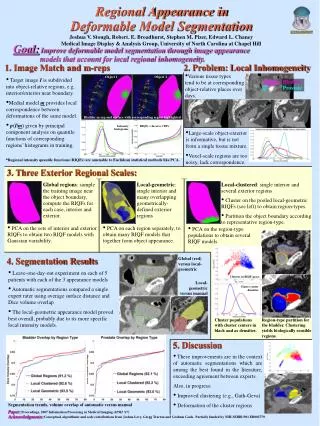
Appearance: Regional Intensity Quantile Functions (RIQFs) [Levina, UC-Berkeley 2002] [Broadhurst et al., ISBI 2006] • Inverse cumulative distribution function. • Suited to PCA. • Regional – local object-relative image extent. • Example: probability density and quantile function.
Global regions Versus geometrically defined local regions Versus regions defined by RIQF clusters. Question: Which Image Match Produces Best Segmentations?
Determine Region Types • Pool RIQFs over all regions and training images. • Fuzzy C-Means Clustering • Example: C= 2 on bladder exterior. [Bezdec 1981]
Eig. 2 Z-score Eig. 1 Z-score Partition the Boundary by Cluster Type • For each patch, choose most popular cluster. • PCA on cluster populations.
Bladder Partition for C= 2 • Confirming evidence • Bladder: mostly fat with prostate and bone • Prostate: dense tissue with bone and bladder, some fat
Experimental Setup Determine local RIQF-types in training data Construct Gaussian models on each type Build a template of optimal types • 5 patient image sets, ~16 images per patient. • UNC RadOnc and William Beaumont, Michigan. • 512 5120.98 0.98 3 mm
Results Summary, Global v Clustered RIQF clustered image match compares favorably with global.
Conclusions: • Local-clustered regions lead to improved segmentations • Already approaching expert quality, exceeding agreement between experts. Future Directions: • Improved clustering • Modeling mixtures • Region shifting
A walk in the projected space of local intensity distributions
Cluster statistics are not specific enough. • Evidence for modeling each patch separately.