Download
1 / 60
600 likes | 690 Views
In the Name of God Computer Networks Chapter 5: The Network Layer. Dr. Shahriar Bijani Shahed University May 2014. Link State Routing. The idea: Discover neighbors, learn their network addresses. Set distance/cost metric: measure the delay or cost to each neighbor .

E N D
In the Name of GodComputer NetworksChapter 5: The Network Layer Dr. ShahriarBijani Shahed University May 2014
Link State Routing The idea: • Discover neighbors, learn their network addresses. • Set distance/cost metric: measure the delay or cost to each neighbor. • Construct packet telling all it has just learned. • Send this packet to (receive packets from) other routers. • Compute shortest path to every other router.
Step1: Discover Neighbors • Sending a special HELLO packet on each point-to-point line. The router on the other end is expected to send back a reply telling who it is. • Modeling the LAN as many point-to-point links increases the size of the topology and leads to wasteful messages; • A better way: consider the LAN as a node itself (a) Nine routers and a broadcast LAN (b) A graph model of (a)
Step 2: measure the Cost (delay) • The most direct way to determine the delay: sending an ECHO packet that the other side is required to send back immediately. • Assumption: delays are symmetric • To optimize the calculation: use the average time
Step 3: Building Link State Packets (a) A network. (b) The link state packets for this network. • The packet includs: • the identity of the sender • a sequence number (Seq.) • the Age • a list of neighbors. • For each neighbor, the delay to that neighbor is given. • Building the link state packets is easy. The hard part is determining when to build them. • periodically: at regular intervals. • Event-based: is to build them when some significant event occurs, such as a line or neighbor going down or coming back up again.
Step 4: Distributing the Link State Packets • The basic distribution algorithm: The fundamental idea is flooding the link state packets. • To control the flood: each packet contains a sequence number that is incremented for each new packet sent. Routers keep track of all the (source router, sequence) pairs they receive. • When a new link state packet arrives, it is checked against the list of packets already seen. • If it is new, it is forwarded on all lines except the one it arrived on. • If it is a duplicate, it is discarded. • If a packet with a sequence number lower than the highest one seen so far ever arrives, it is rejected as being outdated (the router has more recent data).
Step 4: Distributing the Link State Packets The packet buffer of router B • The Age • Add the age of each packet and decrement it once per second. • When the age hits zero, the information from that router is discarded. Normally, a new packet comes in, (e.g. every 10 sec), so router information only times out when a router is down (or 6 consecutive packets have been lost). • The Age field is also decremented by each router during the initial flooding process, to make sure no packet can get lost and live for an indefinite period of time (a packet whose age is zero is discarded).
Step 5: Computing the New Routes • Once a router has accumulated a full set of link state packets, it can construct the entire subnet graph because every link is represented. • Now Dijkstra's algorithm can be run locally to construct the shortest path to all possible destinations.
Hierarchical Routing • The routers are divided into regions: with each router knowing all the detailsabout how to route packets to destinations within its own region, but knowing nothingabout the internal structure of other regions. • For huge networks, a two-level hierarchy may be insufficient; it may be necessary to group the regions into clusters, the clusters into zones, the zones into groups, and so on, until we run out of names for aggregations.
Hierarchical Routing zone cluster region cluster region zone region region region cluster region region region region region region cluster region
Hierarchical Routing • The full routing table for router 1A has 17 entries, as shown in (b). • When routing is done hierarchically, as in (c), there are entries for all the local routers as before, but all other regions have been condensed into a single router, so all traffic for region 2 goes via the 1B -2A line, but the rest of the remote traffic goes via the 1C -3B line. • Hierarchical routing has reduced the table from 17 to 7 entries.
Hierarchical Routing • Unfortunately, these gains in space are not free. • This penalty is in the form of increased path length. • E.g. the best route from 1A to 5C is via region 2, but with hierarchical routing all traffic to region 5 goes via region 3, because that is better for most destinations in region 5.
Broadcast Routing • Broadcasting: Sending a packet to all destinations simultaneously. • The source simply sends a distinct packet to each destination. • Drawbacks: 1) wasteful of bandwidth, 2) requires the source to have a complete list of all destinations. • Flooding. • The problem with flooding as a broadcast technique is that it generates too many packets and consumes too much bandwidth.
Broadcast Routing (Multicast Routing ) • Multi-destination routing. • If this method is used, each packet contains either a list of destinations or a bit map indicating the desired destinations. When a packet arrives at a router, the router checks all the destinations to determine the set of output lines that will be needed. (An output line is needed if it is the best route to at least one of the destinations.) • The router generates a new copy of the packet for each output line to be used and includes in each packet only those destinations that are to use the line. In effect, the destination set is partitioned among the output lines. • After a sufficient number of hops, each packet will carry only one destination and can be treated as a normal packet.
Broadcast Routing • A fourth broadcast algorithm makes explicit use of the sink tree(spanning tree) for the router initiating the broadcast. • If each router knows which of its lines belong to the spanning tree, it can copy an incoming broadcast packet onto all the spanning tree lines except the one it arrived on.
Broadcast Routing • Reverse path forwarding. • When a broadcast packet arrives at a router, the router checks to see if the packet arrived on the line that is normally used for sending packets to the source of the broadcast. • If so, there is an excellent chance that the broadcast packet itself followed the best route from the router and is therefore the first copy to arrive at the router. This being the case, the router forwards copies of it onto all lines except the one it arrived on. • If, however, the broadcast packet arrived on a line other than the preferred one for reaching the source, the packet is discarded as a likely duplicate.
Broadcast Routing • how does the reverse path algorithm works? Reverse path forwarding. (a) A network. (b) A sink tree. (c) The tree built by reverse path forwarding.
Congestion Control Algorithms • Approaches to congestion control • Traffic-aware routing • Admission control • Traffic throttling • Load shedding
Congestion Control Algorithms When too much traffic is offered, congestion sets in and performance degrades sharply.
Flow Control vs. Congestion Control • Congestion control • Make sure the subnet is able to carry the offered traffic • It is a global issue, involving the behavior of all the hosts, all the routers, etc. • Flow Control • Relate to the point-to-point traffic between a given sender and a given receiver.
Flow Control vs. Congestion Control 1000 Gbps Super Computer PC Flow Control 1 Gbps 1 Mbps 1000 Congestion Control 100 Kbps 100 Kbps 1000 PCs 100 Kbps
Congestion Control • Congestion causes • bursty data • insufficient memory • slow processor • low-bandwidth line
General Principles • Open Loop (preventive) • make sure congestion does not occur in the first place • Deciding when to accept new traffic, deciding when to discard packets and which onesand making scheduling decisions at various points in the network. • Closed Loop • monitor the system to detect congestion (where and when) • pass this information to places where action can be taken • adjust system operation to correct the problem
Congestion Control Algorithm Taxonomy (closed loop) • explicit feedback • Packets are sent back from the point of congestion to warn the source. • implicit feedback • The source deduces the existence of congestion by making local observations, such as the acknowledgement time.
Approaches to Congestion Control Timescales of approaches to congestion control
ICMP protocol • error reporting • router “signaling” • IP protocol • addressing conventions • datagram format • packet handling conventions • Routing protocols • path selection • RIP, OSPF, BGP forwarding table THE INTERNET NETWORK LAYER Host, router network layer functions: Transport layer: TCP, UDP Network layer Link layer Physical layer
Internet Network Layer Protocol • The IP (Internal Protocol) Protocol • IP Addressing • Subnets • Internet Control Protocols • The Internet Control Message Protocol (ICMP) • The Address Resolution Protocol (ARP) • The Reverse Address Resolution Protocol (RARP)
The IP Header (IP DATAGRAM FORMAT) 0 4 8 16 19 24 Version IHL Type of service Total length D F M F Identification Fragment offset Time to live Protocol Header checksum 32 bit Source address 32 bit Destination address Options (0 or more words)
The IP Protocol • Version: The current protocol version is 4. • IP Header length (IHL): measured in 32-bit words • for example, without options, its value is 5. • Type of service • Precedence (3 bits): 0 (normal precedence) ~ 7 (network control) • Delay (1 bit): low delay • Throughput (1 bit): high throughput • Reliability (1 bit): high reliability • unused (2 bits)
The IP Protocol • Total length: measured in octets (bytes), including the length of the header and data • Identification: datagram identifier • Flags • unused (1 bit) • DF (1 bit): don’t fragment • MF (1 bit): more fragment • Fragment offset: the offset of this fragment in the original datagram, measured in units of 8 octets
IP FRAGMENTATION & REASSEMBLY • Network links have MTU (max.transfer size) • largest possible link-level frame. • Large IP datagram divided (“fragmented”) within net • one datagram becomes several datagrams • “reassembled” only at final destination • IP header bits used to identify, order related fragments fragmentation: in:1 large out: 3 small reassembly
The IP Protocol • Time to live (TTL): packet lifetime, measured in seconds (hops, in practice) • Protocol: protocol type (e.g., TCP, UDP, ...), RFC 170 • Header checksum • Source IP address • Destination IP address • Options • Padding: to make the header extend to an exact multiple of 32 bits, containing 0
IP Options • Security • to specify how secret the datagram is (usually not used) • Strict source routing • to give the complete path to be followed • Loose source routing • to give a list of routers not to be missed • Record route • to make each router append its IP address • Timestamp • to make each router append its address and timestamp
IP Option Code • Copy (1 bit): • 0: the option will only be copied into the first fragment and not to all fragments • 1: the option should be copied into all fragments • Class (2 bits) • 0: datagram or network control • 1: reserved • 2: debugging and measurement • 3: reserved • Number (5 bits)
IP Addressing • 32 bits long, represented in dotted decimal notation, e.g.: 192.10.6.30 • Network number + Host number • Network numbers are assigned by the NIC (Network Information Center) to avoid conflicts. • All the hosts in a network must have the same network number.
Special IP Addresses A host on this network
223.1.1.2 223.1.2.1 223.1.3.27 223.1.3.1 223.1.3.2 223.1.2.2 IP Addressing 223.1.1.1 • interface: connection between host/router and physical link • router’s typically have multiple interfaces • host typically has one interface • IP addresses associated with each interface 223.1.1.4 223.1.2.9 223.1.1.3 223.1.1.1 = 11011111 00000001 00000001 00000001 223 1 1 1
Network Growth Problem • Problem • Huge administrative overhead • Every time a new network is installed the system administrator has to contact NIC to get a new network number. • Then this number must be announced worldwide. • Solution: To minimize network numbers by sharing one network number among multiple physical networks
223.1.1.0/24 223.1.2.0/24 223.1.3.0/24 Subnets • To determine the subnets, detach each interface from its host or router, creating islands of isolated networks. Each isolated network is called a subnet. Subnet mask: /24
Subnet Addressing • ack like a single network to the outside world • split into several parts for internal use
Subnets A Class B Network • The standard does not restrict subnet masks to select contiguous bits of the address.
host part subnet part 11001000 0001011100010000 00000000 200.23.16.0/23 IP addressing: CIDR CIDR:Classless InterDomain Routing • Subnet portion of address of arbitrary length • address format: a.b.c.d/x, where x is # bits in subnet portion of address
Classless InterDomain Routing (CIDR) • The world was partitioned into zones, each given a portion of the class C address space: • Addresses 194.0.0.0 to 195.255.255.255 for Europe • Addresses 196.0.0.0 to 197.255.255.255 for Others • Addresses 198.0.0.0 to 199.255.255.255 for North America • Addresses 200.0.0.0 to 201.255.255.255 for Central and South America • Addresses 202.0.0.0 to 203.255.255.255 for Asia and Pacific • Addresses 204.0.0.0 to 207.255.255.255 for Others • Addresses 208.0.0.0 to 223.255.255.255 reserved for future use
IP ADDRESSES: HOW TO GET ONE? Q: How does a host get IP address? • Hard-coded by system admin in a file • Windows: control-panel->network->configuration->tcp/ip->properties • UNIX: /etc/rc.config • DHCP:Dynamic Host Configuration Protocol: dynamically get address from a server • “plug-and-play”
E B A DHCP: Dynamic Host Configuration Protocol Goal: allow host to dynamically obtain its IP address from network server when it joins network • Allows reuse of addresses 223.1.2.1 DHCP 223.1.1.1 server 223.1.1.2 223.1.2.9 223.1.1.4 223.1.2.2 arriving DHCP client needs address in this network 223.1.1.3 223.1.3.27 223.1.3.2 223.1.3.1
IP ADDRESSES: HOW TO GET ONE? Q: How does network get subnet part of IP addr? A: It’s allocated portion of its provider ISP’s address space ISP's block 11001000 00010111 00010000 00000000 200.23.16.0/20 Organization 0 11001000 00010111 00010000 00000000 200.23.16.0/23 Organization 1 11001000 00010111 00010010 00000000 200.23.18.0/23 Organization 2 11001000 00010111 00010100 00000000 200.23.20.0/23 ... ….. …. …. Organization 7 11001000 00010111 00011110 00000000 200.23.30.0/23
200.23.16.0/23 200.23.18.0/23 200.23.30.0/23 200.23.20.0/23 . . . . . . HIERARCHICAL ADDRESSING: ROUTE AGGREGATION Hierarchical addressing allows efficient advertisement of routing information: Organization 0 Organization 1 “Send me anything with addresses beginning 200.23.16.0/20” Network Layer Organization 2 ISP Inc. Internet Organization 7 “Send me anything with addresses beginning 199.31.0.0/16” ISPs-R-Us