Download
1 / 31
320 likes | 484 Views
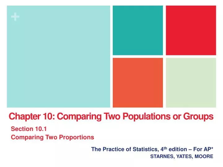
Chapter 10: Comparing Two Populations or Groups. Section 10.1 Comparing Two Proportions. The Practice of Statistics, 4 th edition – For AP* STARNES, YATES, MOORE. Chapter 10 Comparing Two Populations or Groups. 10.1 Comparing Two Proportions 10.2 Comparing Two Means.

E N D
Chapter 10: Comparing Two Populations or Groups Section 10.1 Comparing Two Proportions The Practice of Statistics, 4th edition – For AP* STARNES, YATES, MOORE
Chapter 10Comparing Two Populations or Groups • 10.1 Comparing Two Proportions • 10.2 Comparing Two Means
Section 10.1Comparing Two Proportions Learning Objectives After this section, you should be able to… • DETERMINE whether the conditions for performing inference are met. • CONSTRUCT and INTERPRET a confidence interval to compare two proportions. • PERFORM a significance test to compare two proportions. • INTERPRET the results of inference procedures in a randomized experiment.
Comparing Two Proportions • Introduction Suppose we want to compare the proportions of individuals with a certain characteristic in Population 1 and Population 2. Let’s call these parameters of interest p1 and p2. The ideal strategy is to take a separate random sample from each population and to compare the sample proportions with that characteristic. What if we want to compare the effectiveness of Treatment 1 and Treatment 2 in a completely randomized experiment? This time, the parameters p1 and p2 that we want to compare are the true proportions of successful outcomes for each treatment. We use the proportions of successes in the two treatment groups to make the comparison. Here’s a table that summarizes these two situations.
Comparing Two Proportions • The Sampling Distribution of a Difference Between Two Proportions In Chapter 7, we saw that the sampling distribution of a sample proportion has the following properties: Shape Approximately Normal if np ≥ 10 and n(1 - p) ≥ 10 • To explore the sampling distribution of the difference between two proportions, let’s start with two populations having a known proportion of successes. • At School 1, 70% of students did their homework last night • At School 2, 50% of students did their homework last night. • Suppose the counselor at School 1 takes an SRS of 100 students and records the sample proportion that did their homework. • School 2’s counselor takes an SRS of 200 students and records the sample proportion that did their homework.
Comparing Two Proportions • The Sampling Distribution of a Difference Between Two Proportions Using Fathom software, we generated an SRS of 100 students from School 1 and a separate SRS of 200 students from School 2. The difference in sample proportions was then calculated and plotted. We repeated this process 1000 times. The results are below:
Comparing Two Proportions • The Sampling Distribution of a Difference Between Two Proportions The Sampling Distribution of the Difference Between Sample Proportions Choose an SRS of size n1from Population 1 with proportion of successes p1and an independent SRS of size n2from Population 2 with proportion of successes p2.
Comparing Two Proportions • Example: Who Does More Homework? Suppose that there are two large high schools, each with more than 2000 students, in a certain town. At School 1, 70% of students did their homework last night. Only 50% of the students at School 2 did their homework last night. The counselor at School 1 takes an SRS of 100 students and records the proportion that did homework. School 2’s counselor takes an SRS of 200 students and records the proportion that did homework. School 1’s counselor and School 2’s counselor meet to discuss the results of their homework surveys. After the meeting, they both report to their principals that
Comparing Two Proportions • Example: Who Does More Homework?
Check Your Understanding Suppose I bring two bags of colored goldfish crackers to class. I tell you that Bag 1 has 25% red crackers and Bag 2 has 35% red crackers. Each bag contains more than 500 crackers. Using a paper cup, we take a SRS of 50 crackers from Bag 1 and a separate SRS of 40 crackers from Bag 2. Let p hat 1 – p hat 2 be the difference in the sample proportions of red crackers. 1. What is the shape of the sampling distribution of p hat 1 – p hat 2 ? 2. Find the mean and standard deviation of the sampling distribution. 3. Find the probability that p hat 1 – p hat 2 is less than -0.02. 4. Based on your answer to Question 3, would you be surprised if the difference in the proportion of red crackers in the two samples was p hat 1 – p hat 2 = -0.02? Explain
Assignment #1,3,5
Comparing Two Proportions • Confidence Intervals for p1 – p2 If the Normal condition is met, we find the critical value z* for the given confidence level from the standard Normal curve. Our confidence interval for p1 – p2is:
Comparing Two Proportions • Two-Sample z Interval for p1 – p2 Two-Sample zInterval for a Difference Between Proportions
Comparing Two Proportions • Example: Teens and Adults on Social Networks As part of the Pew Internet and American Life Project, researchers conducted two surveys in late 2009. The first survey asked a random sample of 800 U.S. teens about their use of social media and the Internet. A second survey posed similar questions to a random sample of 2253 U.S. adults. In these two studies, 73% of teens and 47% of adults said that they use social-networking sites. Use these results to construct and interpret a 95% confidence interval for the difference between the proportion of all U.S. teens and adults who use social-networking sites. State: Our parameters of interest are p1= the proportion of all U.S. teens who use social networking sites and p2= the proportion of all U.S. adults who use social-networking sites. We want to estimate the difference p1 – p2at a 95% confidence level. • Plan: We should use a two-sample z interval for p1 – p2if the conditions are satisfied. • Random The data come from a random sample of 800 U.S. teens and a separate random sample of 2253 U.S. adults. • Normal We check the counts of “successes” and “failures” and note the Normal condition is met since they are all at least 10: • Independent We clearly have two independent samples—one of teens and one of adults. Individual responses in the two samples also have to be independent. The researchers are sampling without replacement, so we check the 10% condition: there are at least 10(800) = 8000 U.S. teens and at least 10(2253) = 22,530 U.S. adults.
Do: Since the conditions are satisfied, we can construct a two-sample z interval for the difference p1 – p2. Comparing Two Proportions • Example: Teens and Adults on Social Networks Conclude: We are 95% confident that the interval from 0.223 to 0.297 captures the true difference in the proportion of all U.S. teens and adults who use social-networking sites. This interval suggests that more teens than adults in the United States engage in social networking by between 22.3 and 29.7 percentage points.
Check Your Understanding Are teens or adults more likely to go online daily? The Pew Internet and American Life Project asked a random sample of 800 teens and a separate random sample of 2253 adults how often they use the Internet. In these two surveys, 63% of the teens and 68% of the adults said that they go online every day. Construct and interpret a 90% confidence interval for p1-p2
Assignment #7,9,11,13
An observed difference between two sample proportions can reflect an actual difference in the parameters, or it may just be due to chance variation in random sampling or random assignment. Significance tests help us decide which explanation makes more sense. The null hypothesis has the general form H0: p1 - p2= hypothesized value We’ll restrict ourselves to situations in which the hypothesized difference is 0. Then the null hypothesis says that there is no difference between the two parameters: H0: p1 - p2 = 0 or, alternatively, H0: p1 = p2 The alternative hypothesis says what kind of difference we expect. Ha: p1 - p2 > 0, Ha: p1 - p2 < 0, or Ha: p1 - p2 ≠ 0 Comparing Two Proportions • Significance Tests for p1 – p2 If the Random, Normal, and Independent conditions are met, we can proceed with calculations.
Comparing Two Proportions • Significance Tests for p1 – p2 If H0: p1 = p2is true, the two parameters are the same. We call their common value p. But now we need a way to estimate p, so it makes sense to combine the data from the two samples. This pooled (or combined) sample proportion is:
Comparing Two Proportions • Two-Sample z Test for The Difference Between Two Proportions If the following conditions are met, we can proceed with a two-sample z test for the difference between two proportions: Two-Sample z Test for the Difference Between Proportions
Comparing Two Proportions • Example: Hungry Children • Researchers designed a survey to compare the proportions of children who come to school without eating breakfast in two low-income elementary schools. An SRS of 80 students from School 1 found that 19 had not eaten breakfast. At School 2, an SRS of 150 students included 26 who had not had breakfast. More than 1500 students attend each school. Do these data give convincing evidence of a difference in the population proportions? Carry out a significance test at the α= 0.05 level to support your answer. State: Our hypotheses are H0: p1 - p2 = 0 Ha: p1 - p2 ≠ 0 where p1= the true proportion of students at School 1 who did not eat breakfast, and p2= the true proportion of students at School 2 who did not eat breakfast. • Plan: We should perform a two-sample z test for p1 – p2if the conditions are satisfied. • Random The data were produced using two simple random samples—of 80 students from School 1 and 150 students from School 2. • Normal We check the counts of “successes” and “failures” and note the Normal condition is met since they are all at least 10: • Independent We clearly have two independent samples—one from each school. Individual responses in the two samples also have to be independent. The researchers are sampling without replacement, so we check the 10% condition: there are at least 10(80) = 800 students at School 1 and at least 10(150) = 1500 students at School 2.
Do: Since the conditions are satisfied, we can perform a two-sample z test for the difference p1 – p2. Comparing Two Proportions • Example: Hungry Children P-value Using Table A or normalcdf, the desired P-value is 2P(z ≥ 1.17) = 2(1 - 0.8790) = 0.2420. Conclude: Since our P-value, 0.2420, is greater than the chosen significance level of α = 0.05,we fail to reject H0. There is not sufficient evidence to conclude that the proportions of students at the two schools who didn’t eat breakfast are different.
Comparing Two Proportions • Example: Significance Test in an Experiment • High levels of cholesterol in the blood are associated with higher risk of heart attacks. Will using a drug to lower blood cholesterol reduce heart attacks? The Helsinki Heart Study recruited middle-aged men with high cholesterol but no history of other serious medical problems to investigate this question. The volunteer subjects were assigned at random to one of two treatments: 2051 men took the drug gemfibrozil to reduce their cholesterol levels, and a control group of 2030 men took a placebo. During the next five years, 56 men in the gemfibrozil group and 84 men in the placebo group had heart attacks. Is the apparent benefit of gemfibrozil statistically significant? Perform an appropriate test to find out. State: Our hypotheses are H0: p1 - p2 = 0 OR H0: p1 = p2 Ha: p1 - p2 < 0 Ha: p1 < p2 where p1is the actual heart attack rate for middle-aged men like the ones in this study who take gemfibrozil, and p2is the actual heart attack rate for middle-aged men like the ones in this study who take only a placebo. No significance level was specified, so we’ll use α = 0.01 to reduce the risk of making a Type I error (concluding that gemfibrozil reduces heart attack risk when it actually doesn’t).
Plan: We should perform a two-sample z test for p1 – p2if the conditions are satisfied. • Random The data come from two groups in a randomized experiment • Normal The number of successes (heart attacks!) and failures in the two groups are 56, 1995, 84, and 1946. These are all at least 10, so the Normal condition is met. • Independent Due to the random assignment, these two groups of men can be viewed as independent. Individual observations in each group should also be independent: knowing whether one subject has a heart attack gives no information about whether another subject does. Comparing Two Proportions • Example: Cholesterol and Heart Attacks Do: Since the conditions are satisfied, we can perform a two-sample z test for the difference p1 – p2. Conclude: Since the P-value, 0.0068, is less than 0.01, the results are statistically significant at the α = 0.01 level. We can reject H0and conclude that there is convincing evidence of a lower heart attack rate for middle-aged men like these who take gemfibrozil than for those who take only a placebo. P-value Using Table A or normalcdf, the desired P-value is 0.0068
Check Your Understanding To study the long-term effects of preschool programs for poor children, researchers designed an experiment. They recruited 123 children who had never attended preschool from low-income families in Michigan. Researchers randomly assigned 62 of the children to attend preschool (paid for by the study budget) and the other 61 to serve as a control group who would not go to preschool. One response variable of interest was the need for social services as adults. In the past 10 years, 38 children in the preschool group and 49 in the control group have needed social services. 1. Does this study provide convincing evidence that preschool reduces the later need for social services? Carry out an appropriate test to help answer this question.
Check Your Understanding 2. The Minitab output below gives a 95% confidence interval for p1-p2. Interpret this interval in context. Then explain what additional information the confidence interval provides.
Assignment #15,17,21,23
Section 10.1Comparing Two Proportions Summary In this section, we learned that… • Choose an SRS of size n1from Population 1 with proportion of successes p1and an independent SRS of size n2from Population 2 with proportion of successes p2. • Confidence intervals and tests to compare the proportions p1and p2of successes for two populations or treatments are based on the difference between the sample proportions. • When the Random, Normal, and Independent conditions are met, we can use two-sample z procedures to estimate and test claims about p1 - p2.
Section 10.1Comparing Two Proportions Summary In this section, we learned that… • The conditions for two-sample z procedures are: • An approximate level C confidence interval for p1 - p2is where z* is the standard Normal critical value. This is called a two-sample z interval for p1 - p2.
Section 10.1Comparing Two Proportions Summary In this section, we learned that… • Significance tests of H0: p1 - p2= 0 use the pooled (combined) sample proportion • The two-sample z test for p1- p2uses the test statistic with P-values calculated from the standard Normal distribution. • Inference about the difference p1 - p2in the effectiveness of two treatments in a completely randomized experiment is based on the randomization distribution of the difference of sample proportions. When the Random, Normal, and Independent conditions are met, our usual inference procedures based on the sampling distribution will be approximately correct.
Looking Ahead… In the next Section… • We’ll learn how to compare two population means. • We’ll learn about • The sampling distribution for the difference of means • The two-sample t procedures • Comparing two means from raw data and randomized experiments • Interpreting computer output for two-sample t procedures