Download
1 / 47
520 likes | 1.99k Views
Introduction to Wavelet Transform and Image Compression. Student: Kang-Hua Hsu 徐康華 Advisor: Jian-Jiun Ding 丁建均 E-mail: r96942097@ntu.edu.tw Graduate Institute of Communication Engineering National Taiwan University, Taipei, Taiwan, ROC. DISP@MD531. Outline (1). Introduction

E N D
Introduction to Wavelet Transform and Image Compression Student: Kang-Hua Hsu徐康華 Advisor: Jian-Jiun Ding 丁建均 E-mail: r96942097@ntu.edu.tw Graduate Institute of Communication Engineering National Taiwan University, Taipei, Taiwan, ROC DISP@MD531
Outline (1) • Introduction • Multiresolution Analysis (MRA)- Subband Coding- Haar Transform- Multiresolution Expansion • Wavelet Transform (WT)- Continuous WT- Discrete WT- Fast WT- 2-D WT • Wavelet Packets • Fundamentals of Image Compression- Coding Redundancy- Interpixel Redundancy- Psychovisual Redundancy- Image Compression Model DISP@MD531
Outline (2) • Lossless Compression- Variable-Length Coding- Bit-plane Coding- Lossless Predictive Coding • Lossy Compression- Lossy Predictive Coding- Transform Coding- Wavelet Coding • Conclusion • Reference DISP@MD531
Introduction(1)-WT v.s FT Bases of the • FT: time-unlimited weighted sinusoids with different frequencies. No temporal information. • WT: limited duration small waves with varying frequencies, which are called wavelets. WTs contain the temporal time information. Thus, the WT is more adaptive. DISP@MD531
Introduction(2)-WT v.s TFA • Temporal information is related to the time-frequency analysis. • The time-frequency analysis is constrained by the Heisenberg uncertainty principal. • Compare tiles in a time-frequency plane (Heisenberg cell): DISP@MD531
Introduction(3)-MRA • It represents and analyzes signals at more than one resolution. • 2 related operations with ties to MRA: • Subband coding • Haar transform • MRA is just a concept, and the wavelet-based transformation is one method to implement it. DISP@MD531
Introduction(4)-WT • The WT can be classified according to the of its input and output. • Continuous WT (CWT) • Discrete WT (DWT) • 1-D 2-D transform (for image processing) • DWT Fast WT (FWT) recursive relation of the coefficients DISP@MD531
MRA-Subband Coding(1) • Since the bandwidth of the resulting subbands is smaller than that of the original image, the subbands can be downsampled without loss of information. • We wish to select so that the input can be perfectly reconstructed. • Biorthogonal • Orthonormal DISP@MD531
MRA-Subband Coding(2) • Biorthogonal filter bank: • Orthonormal (it’s also biorthogonal) filet bank: : time-reversed relation ,where 2K denotes the number of coefficients in each filter. • The other 3 filters can be obtained from one prototype filter. DISP@MD531
MRA-Subband Coding(3) • 1-D to 2-D: 1-D two-band subband coding to the rows and then to the columns of the original image. • Where a is the approximation (Its histogram is scattered, and thus lowly compressible.) and d means detail (highly compressible because their histogram is centralized, and thus easily to be modeled). FWT can be implemented by subband coding! DISP@MD531
Haar Transform will put the lower frequency components of X at the top-left corner of Y. This is similar to the DWT. This implies the resolution (frequency) and location (time). DISP@MD531
Multiresolution Expansions(1) • , : the real-valued expansion coefficients. , : the real-valued expansion functions. • Scaling function : span the approximation of the signal. • : this is the reason of it’s name. • If we define , then • , : scaling function coefficients DISP@MD531
Multiresolution Expansions(2) • 4 requirements of the scaling function: • The scaling function is orthogonal to its integer translates. • The subspaces spanned by the scaling function at low scales are nested within those spanned at higher scales. • The only function that is common to all is . • Any function can be represented with arbitrary coarse resolution, because the coarser portions can be represented by the finer portions. DISP@MD531
Multiresolution Expansions(3) • The wavelet function : spans difference between any two adjacent scaling subspaces, and . • span the subspace . DISP@MD531
Multiresolution Expansions(4) • , : wavelet function coefficients • Relation between the scaling coefficients and the wavelet coefficients: This is similar to the relation between the impulse response of the analysis and synthesis filters in page 11. There is time-reverse relation in both cases. DISP@MD531
CWT • The definition of the CWT is • Continuous input to a continuous output with 2 continuous variables, translation and scaling. • Inverse transform: It’s guaranteed to be reversible if the admissibility criterion is satisfied. • Hard to implement! DISP@MD531
DWT(1) : arbitrary starting scale • wavelet series expansion: : approximation or scaling coefficients : detail or wavelet coefficients This is still the continuous case. If we change the integral to summation, the DWT is then developed. DISP@MD531
DWT(2) The coefficients measure the similarity (in linear algebra, the orthogonal projection) of with basis functions and . DISP@MD531
FWT(1) By the 2 relations we mention in subband coding, We can then have DISP@MD531
FWT(2) When the input is the samples of a function or an image, we can exploit the relation of the adjacent scale coefficients to obtain all of the scaling and wavelet coefficients without defining the scaling and wavelet functions. DISP@MD531
FWT(3) FWT resembles the two-band subband coding scheme! • The constraints for perfect reconstruction is the same as in the subband coding. DISP@MD531
2-D WT(1) 1-D (row) 2-D 1-D (column) These wavelets have directional sensitivity naturally. DISP@MD531
2-D WT(2) Note that the upmost-leftmost subimage is similar to the original image due to the energy of an image is usually distributed around lower band. DISP@MD531
Wavelet Packets A wavelet packet is a more flexible decomposition. DISP@MD531
Fundamentals of Image Compression(1) • 3 kinds of redundancies in an image: • Coding redundancy • Interpixel redundancy • Psychovisual redundancy Image compression is achieved when the redundancies were reduced or eliminated. Goal: To convey the same information with least amount of data (bits). DISP@MD531
Fundamentals of Image Compression(2) • Image compression can be classified to • Lossless(error-free, without distortion after reconstructed) • Lossy • Information theory is an important tool . Data Information : information is “carried” by the data. DISP@MD531
Fundamentals of Image Compression(3) • Evaluation of the lossless compression: • Compression ratio : • Relative data redundancy : • Evaluation of the lossy compression: • root-mean-square (rms) error DISP@MD531
Coding Redundancy If there is a set of codeword to represent the original data with less bits, the original data is said to have coding redundancy. • We can obtain the probable information from the histogram of the original image. • Variable-length coding: assign shorter codeword to more probable gray level. DISP@MD531
Interpixel Redundancy(1) Interpixel redundancy is resulted from the correlation between neighboring pixels. • Because the value of any given pixel can be reasonably predicted from the value of its neighbors, the information carried by individual pixels is relatively small. DISP@MD531
Interpixel Redundancy(2) • To reduce interpixel redundancy, the original image will be transformed to a more efficient and nonvisual format. This transformation is called mapping. • Run-length coding. Ex. 10000000 1,111 • Difference coding. 7 0s DISP@MD531
Psychovisual Redundancy Humans don’t respond with equal importance to every pixel. • For example, the edges are more noticeable for us. • Information loss! • We truncate or coarsely quantize the gray levels (or coefficients) that will not significantly impair the perceived image quality. • The animation take advantage of the persistence of vision to reduce the scanning rate. DISP@MD531
Image Compression Model • The quantizer is not necessary. • The mapper would • reduce the interpixel redundancy to compress directly, such as exploiting the run-length coding.or • make it more accessible for compression in the later stage, for example, the DCT or the DWT coefficients are good candidates for quantization stage. DISP@MD531
Lossless Compression • No quantizer involves in the compression procedure. • Generally, the compression ratios range from 2 to 10. • Trade-off relation between the compression ratio and the computational complexity. It can be reconstructed without distortion. DISP@MD531
Variable-Length Coding It assigns fewer bits to the more probable gray levels than to the less probable ones. • It merely reduces the coding redundancy. • Ex. Huffman coding DISP@MD531
Bit-plane Coding A monochrome or colorful image is decomposed into a series of binary images (that is, bit planes), and then they are compressed by a binary compression method. • It reduces the interpixel redundancy. DISP@MD531
Lossless Predictive Coding It encodes the difference between the actual and predicted value of that pixel. • It reduces the interpixel redundancies of closely spaced pixels. • The ability to attack the redundancy depends on the predictor. DISP@MD531
Lossy Compression It can not be reconstructed without distortion due to the sacrificed accuracy. • It exploits the quantizer. • Its compression ratios range from 10 to 100 (much more than the lossless case’s). • Trade-off relation between the reconstruction accuracy and compression performance. DISP@MD531
Lossy Predictive Coding It is just a lossless predictive coding containing a quantizer. • It exploits the quantizer. • Its compression ratios range from 10 to 100 (much more than the lossless case’s). • The quantizer is designed based on the purpose for minimizing the quantization error. • Trade-off relation between the quantizer complexity and less quantization error. • Delta modulation (DM) is an easy example exploiting the oversampling and 1-bit quantizer. DISP@MD531
Transform Coding(1) Most of the information is included among a small number of the transformed coefficients. Thus, we truncate or coarsely quantize the coefficients including little information. • The goal of the transformation is to pack as much information as possible into the smallest number of transform coefficients. • Compression is achieved during the quantization of the transformed coefficients, not during the transformation. DISP@MD531
Transform Coding(2) • More truncated coefficients Higher compression ratio, but the rms error between the reconstructed image and the original one would also increase. • Every stage can be adapted to local image content. • Choosing the transform: • Information packing ability • Computational complexity needed Practical! DISP@MD531
Transform Coding(3) • Disadvantage: Blocking artifact when highly compressed (this causes errors) due to subdivision. • Size of the subimage: • Size increase: higher compression ratio, computational complexity, and bigger block size. ? ? ? ? How to solve the blocking artifact problem? Using the WT! ? ? ? DISP@MD531
Wavelet Coding(1) Wavelet coding is not only the transforming coding exploiting the wavelet transform------No subdivision! • No subdivision due to: • Computationally efficient (FWT) • Limited-duration basis functions. Avoiding the blocking artifact! DISP@MD531
Wavelet Coding(2) • We only truncate the detail coefficients. • The decomposition level: the initial decompositions would draw out the majority of details. Too many decompositions is just wasting time. DISP@MD531
Wavelet Coding(3) • Quantization with dead zone threshold: set a threshold to truncate the detail coefficients that are smaller than the threshold. DISP@MD531
Conclusion The WT is a powerful tool to analyze signals. There are many applications of the WT, such as image compression. However, most of them are still not adopted now due to some disadvantage. Our future work is to improve them. For example, we could improve the adaptive transform coding, including the shape of the subimages, the selection of transformation, and the quantizer design. They are all hot topics to be studied. DISP@MD531
Reference [1] R.C Gonzalez, R.E Woods, Digital Image Processing, 2nd edition, Prentice Hall, 2002. [2] J.C Goswami, A.K Chan, Fundamentals of Wavelets, John Wiley & Sons, New York, 1999. [3] Contributors of the Wikipedia, “Arithmetic coding”, available in http://en.wikipedia.org/wiki/Arithmetic_coding. [4] Contributors of the Wikipedia, “Lempel-Ziv-Welch”, available in http://en.wikipedia.org/wiki/Lempel-Ziv-Welch. [5] S. Haykin, Communication System, 4th edition, John Wiley & Sons, New York, 2001. DISP@MD531