Download

1 / 29
300 likes | 320 Views
Chapters 8. Overview of Queuing Analysis. Projected vs. Actual Response Time. Introduction- Motivation. How to analyze changes in network workloads? (i.e., a helpful tool to use) Analysis of system (network) load and performance characteristics response time throughput

E N D
Chapters 8 Overview of Queuing Analysis
Projected vs. Actual Response Time Chapter 8 Overview of Queuing Analysis
Introduction- Motivation • How to analyze changes in network workloads? (i.e., a helpful tool to use) • Analysis of system (network) load and performance characteristics • response time • throughput • Performance tradeoffs are often not intuitive • Queuing theory, although mathematically complex, often makes analysis very straightforward Chapter 8 Overview of Queuing Analysis
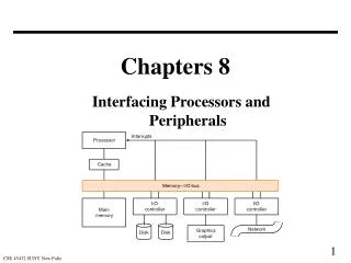
Items Lost Single-Server Queuing System Queuing System (Delay Box) Items Arriving (message, packet, cell) Items Departing Chapter 8 Overview of Queuing Analysis
Parameters for Single-Server Queuing System • Comments, assuming queue has infinite capacity: • At = 1, server is working 100% of the time (saturated), so items are queued (delayed) until they can be served. Departures remain constant (for same L). • Traffic intensity, u = L/R. Note that Ts = L/R, so: • max = 1 / Ts = 1 / (L/R) is the theoretical maximum arrival rate, and that • Lmax/R = u = 1 at the theoretical maximum arrival rate Chapter 8 Overview of Queuing Analysis
The Fundamental Task of Queuing Analysis • Given: • Arrival rate, • Service time, Ts • Number of servers, N • Determine: • Items waiting, w • Waiting time, Tw • Items queued, r • Residence time, Tr Chapter 8 Overview of Queuing Analysis
Queuing Process - Example Depth of the Queue General Expression: TRn+1 = TSn+1 + MAX[0, Dn – An+1] Chapter 8 Overview of Queuing Analysis
General Characteristics of Network Queuing Models • Item population • generally assumed to be infinite therefore, arrival rate is persistent • Queue size • infinite, therefore no loss • finite, more practical, but often immaterial • Dispatching discipline • FIFO, typical • LIFO • Relative/Preferential, based on QoS Chapter 8 Overview of Queuing Analysis
Multiserver Queuing System • Comments: • Assuming N identical servers, and is the utilization of each server. • Then, N is the utilization of the entire system, and the maximum utilization is N x 100%. • Therefore, the maximum supportable arrival rate that the system can handle is: max = N / Ts Chapter 8 Overview of Queuing Analysis
Multiple Single-Server Queuing Systems Chapter 8 Overview of Queuing Analysis
Ts N Basic Queuing Relationships Chapter 8 Overview of Queuing Analysis
Kendall’s notation • Notation is X/Y/N, where: X is distribution of interarrival times Y is distribution of service times N is the number of servers • Common distributions • G = general distribution if interarrival times or service times • GI = general distribution of interarrival time with the restriction that they are independent • M = exponential distribution of interarrival times (Poisson arrivals – p. 167) and service times • D = deterministic arrivals or fixed length service M/M/1? M/D/1? Chapter 8 Overview of Queuing Analysis
Important Formulas for Single-Server Queuing Systems Note Coefficient of variation: if Ts = Ts => exponential if Ts = 0 => constant Chapter 8 Overview of Queuing Analysis
Mean Number of Items in System (r)- Single-Server Queuing Ts/Ts = Coefficient of variation M/M/1 M/D/1 Chapter 8 Overview of Queuing Analysis
Mean Residence Time – (Tr) Single-Server Queuing M/M/1 M/D/1 Chapter 8 Overview of Queuing Analysis
Multiple Server Queuing Systems Multiserver Queuing System Multiple Single-Server Queuing System Chapter 8 Overview of Queuing Analysis
Important Formulas for Multiserver Queuing Note: Useful only in M/M/N case, with equal service times at all N servers. Chapter 8 Overview of Queuing Analysis
Multiple Server Queuing Example (p. 203) Single server M/M/1 (2nd Floor) Multiserver M/M/? (2nd Floor) Multiple Single server M/M/1 (1st Floor) M/M/1 (2nd Floor) M/M/1 (3rd Floor) Chapter 8 Overview of Queuing Analysis
MultiServer vs. Multiple Single-Server Queuing System Comparison (from example problem, pp. 203-204) Single server case (M/M/1): Single server utilization: = 10 engineers x 0.5 hours each / 8 hour work day = 5/8 = .625 Average time waiting: Tw = Ts / 1 - = 0.625 x 30 / .375 = 50 minutes Arrival rate: = 10 engineers per 8 hours = 10/480 = 0.021 engineers/minute 90th percentile waiting time: mTw(90) = Tw/ x ln(10) = 146.6 minutes Average number of engineers waiting: w = Tw = 0.021 x 50 = 1.0416 engineers Chapter 8 Overview of Queuing Analysis
… Internet • Determine: • Tr= Ts / (1-) = .12sec/.4 = .3 sec • r = / (1-) = .6/.4 = 1.5 packets • 3. mr(90) = - 1 = 3.5 packets • mr(95) = - 1 = 4.8 packets For 3 & 4, use: mr(y) = - 1 ln(1-.90) ln (.6) ln(1-.95) ln (.6) ln(1 – y/100) ln Example: Router Queuing • = 5 packets/sec L = 144 octets 9600 bps • From data provided: • Ts = L/R = (144x8)/9600 = .12sec • = Ts = 5 packets/sec x .12sec = .6 Chapter 8 Overview of Queuing Analysis
r Priorities in Queues – Two priority classes Chapter 8 Overview of Queuing Analysis
Tr 64Kbps Find the average Queuing Delay (Tr) through the router: Tr1 = Ts1 + = .01 + = 0.098 sec Tr2 = Ts2 + = .1 + = 0. 833 sec Tr = Tr1 + Tr2 = .5 x .098 + .5 x .833 = 0.4655 sec 1Ts 1 + 2 Ts 2 1 - 1 2 .08 x .01 + .8 x .1 1-.08 1 .098- .01 1 - .88 Tr 1 -Ts 1 1 - Priorities in Queues – Example • Router queue services two packet sizes: • Long = 800 octets • Short = 80 octets • Lengths exponentially distributed • Arrival rates are equal, 8packets/sec • Link transmission rate is 64Kbps • Short packets are priority 1, • Longer packets are priority 2 From data above, calculate: Ts 1 = Lshort/R = (80 x 8) / 64000 = .01 sec Ts 2 = Llong/R = (800 x 8) / 64000 = .1 sec 1 = Ts 1 = 8 x 0.01 = 0.08 2 = Ts 2 = 8 x 0.1 = 0.8 = 1 +2 = 0.88 Chapter 8 Overview of Queuing Analysis
Network of Queues Chapter 8 Overview of Queuing Analysis
Elements of Queuing Networks Chapter 8 Overview of Queuing Analysis
Queuing Networks Chapter 8 Overview of Queuing Analysis
Jackson’s Theorem and Queuing Networks • Assumptions: • the queuing network has m nodes, each providing exponential service • items arriving from outside the system at any node arrive with a Poisson rate • once served at a node, an item moves immediately to another with a fixed probability, or leaves the network • Jackson’s Theorem states: • each node is an independent queuing system with Poisson inputs determined by partitioning, merging and tandem queuing principles • each node can be analyzed separately using the M/M/1 or M/M/N models • mean delays at each node can be added to determine mean system (network) delays Chapter 8 Overview of Queuing Analysis
Internal load: = i where: = total on all links in network i = load on link i L = total number of links L i=1 • Note: • Internal > offered load • Average length for all paths: • E[number of links in path] = / • Average number of item waiting • and being served in link i: ri = i Tri • Average delay of packets sent • through the network is: • T = • where: M is average packet length and • Ri is the data rate on link i External load, offered to network: = jk where: = total workload in packets/sec jk = workload between source j and destination k N = total number of (external) sources and destinations N N j=1 k=2 Mi Ri - Mi 1 L i=1 Jackson’s Theorem - Application in Packet Switched Networks Packet Switched Network Chapter 8 Overview of Queuing Analysis
Estimating Model Parameters • To enable queuing analysis using these models, we must estimate certain parameters: • Mean and standard deviation of arrival rate • Mean and standard deviation of service time (or, packet size) • Typically, these estimates use sample measurements taken from an existing system Chapter 8 Overview of Queuing Analysis
Sampling: • The mean is generally the most important quantity to estimate: • () = Xi • Sample mean is itself a random variable • Central Limit Theorem: the probability distribution tends to normal as sample size, N, increases for virtually all underlying distributions • The mean and variance of X can be calculated as: • E[]= E[X] = • Var[]= 2x/N 1 N N i = 1 Sample Means for Exponential Distribution Chapter 8 Overview of Queuing Analysis