Download
1 / 41
410 likes | 512 Views
Behavior of Aggregate Demand. Increase/Decrease Shift Right/Left Recessionary/Inflationary Gaps. Major Questions to Address. What are the components of aggregate demand? What determines the level of spending for each component? Will there be enough demand to maintain full employment?.

E N D
Behavior of Aggregate Demand Increase/Decrease Shift Right/Left Recessionary/Inflationary Gaps
Major Questions to Address • What are the components of aggregate demand? • What determines the level of spending for each component? • Will there be enough demand to maintain full employment?
Four Components of Aggregate Demand • Consumption (C) • Investment (I) • Government spending (G) • Net exports (X - IM)
ConsumptionBig but Stable Two Components Autonomous Consumption Income-Dependent (Induced) Consumption
Income and Consumption • By definition, all disposable income is either consumed (spent ) or saved (not spent). Disposable income = Consumption + Saving YD = C + S
2000 1999 C = YD 1998 1997 1996 1995 1994 1993 1992 1991 1990 1989 1988 1987 1986 1985 1984 1983 1982 1981 1980 Actual consumer spending 45° U.S. Consumption and Income $7000 6000 5000 4000 CONSUMPTION (billions of dollars per year) 3000 2000 1000 0 $1000 2000 3000 4000 5000 6000 7000 DISPOSABLE INCOME (billions of dollars per year)
The Marginal Propensity to Consume • The marginal propensity to consume(MPC) is the fraction of each additional (marginal) dollar of disposable income spent on consumption.
Marginal Propensity to Save • The marginal propensity to save (MPS) is the fraction of each additional (marginal) dollar of disposable income not spent on consumption. MPS = 1 – MPC
The Consumption Function • The consumption function is a mathematical relationship that helps to predict consumer behavior.
The consumption function provides a precise basis for predicting how changes in income (YD) effect consumer spending (C). C = a + bYD where: C = current consumption a = autonomous consumption (constant) b = marginal propensity to consume (slope) YD= disposable income
Autonomous Consumption • The non income determinants of consumption include • expectations, • wealth, • credit, • taxes, • and price levels.
$125 Consumption Function $400 C = YD E Saving D C Dissaving Consumption Function C = $50 + 0.75YD B G A $50 100 150 200 250 300 350 400 450
C = a2 + bYD C = a1 + bYD CONSUMPTION (C) (dollars per year) a2 a1 0 DISPOSABLE INCOME(dollars per year) Shift in the Consumption Function Increased confidence
Expenditure Price Level Shift = f2 – f1 C2 f2 C1 P1 f1 AD2 AD1 Y0 Income Q1 Q2 Real Output AD Effects of Consumption Shifts
InvestmentSmall but Volatile • Investment are expenditures on new plant, equipment, and structures (capital) in a given time period, plus changes in business inventories. • investment depends on: • Expectations. • Interest rates. • Technology and innovation.
11 10 Better expectations 9 C A 8 7 B 6 I2 Interest Rate (percent per year) 5 Initial expectations 4 11 3 Worse expectations I3 2 1 0 100 200 300 400 500 Planned Investment Spending (billions of dollars per year) Investment Demand
Government Spending • The government sector (federal, state, and local) currently spends over $2 trillion a year on goods and services. • Government spending decisions are made independently of current income.
Net Exports • Net exports can be both uncertain and unstable, creating further shifts of aggregate demand.
GDP Gaps • equilibrium GDP may not occur at full-employment GDP. • Equilibrium GDP is the value of total output (real GDP) produced at macro equilibrium (AS=AD). • Full-employment GDP is the value of total output (real GDP) produced at full employment.
Recessionary GDP Gap 130 AD AS 120 110 100 E 90 Recessionary GDP gap 80 70 65 60 9 10 11 12 13 3 4 5 6 7 8 Full-employment GDP REAL GDP Equilibrium GDP
PRICE LEVEL AS AD3 E3 P3 E1 P* QE3 Q3 QF Inflationary GDP Gap Demand-pull inflation: (too much AD)
The Keynesian Cross The Keynesian cross relates aggregate expenditure to total income (output). At equilibrium, aggregate expenditure equals income (output).
Aggregate Expenditures • Aggregate expenditures are the rate of total expenditure desired at alternative levels of income, ceteris paribus, at a given price level • Aggregate expenditures is the sum of C, I, G, and NX, at a given price level
ZF $3000 2350 CF Total output 2000 Output not purchased by consumers Expenditure 1500 1000 Consumption function (C)= $100 + 0.75YD 500 YF 45° 0 1000 2000 3000 Income (Output) The Consumption Shortfall
Aggregate Expenditures includes Nonconsumer Spending • Investors, governments, and net export buyers add to consumer spending to equal aggregate expenditure.
Expenditure Equilibrium • Equilibrium is the point where aggregate expenditure and 45 degree lines meet. • Recall that real GDP can be calculated as the value of final goods and services, or as the payments to all inputs in its production. • In essence real output = income
Expenditure Equilibrium $3500 AE = Y 3000 2500 Equilibrium 2000 E Expenditure 1500 Aggregate expenditure 1000 500 YE 45° 0 $500 1000 1500 2000 2500 3000 Income (Output) (billions of dollars per year)
When AE > Y, inventories depleting, signals expansion • When Y > AE, inventories increasing, signals contraction
Aggregate Expenditure at different price levels Plots out Aggregate Demand Wealth, Int’l Trade and Money Demand Effects
Aggregate Expenditures C + I + G + NX YD= Y – tY = (1-t)Y C = a + mpcYD = a + mpc (1-t)Y I = I – di G = G NX = NX AE=a + I – di + G + NX + mpc (1-t)Y AE = AE + mpc (1-t)Y
Changes to Autonomous Expenditure Autonomous spending • Autonomous Consumption • Investment • Gov’t Spending • Net Exports Shifts Aggregate Expenditure Up or Down Shifts Aggregate Demand Right or Left
AE + mpc (1-t) Y Aggregate Expenditures AE C = a + mpc (1-t) Y G I - di NX Y* Y real output/Income
AE0 + mpc (1-t) Y Aggregate Expenditures AE1 AE 0 Y0 Y1 Y real output/Income AE1 + mpc (1-t) Y
AE1 AE 0 An increase in autonomous aggregate expenditures has a much larger increase in real output/income. Multiplier Effect Y0 Y1
Multiplier Effect • An increase in autonomous expenditures increases income by a like amount • With the increase in income, there is an increase in induced consumption. • The increase in consumption, again increases income. • The increase in consumption diminishes at each step due to savings and taxes.
Deriving the Multiplier ΔY =ΔAE + mpc(1-t)ΔAE + mpc(1-t)[mpc(1-t)ΔAE] +mpc(1-t)[mpc(1-t)mpc(1-t)ΔAE] +…… ΔY =ΔAE{1 + mpc(1-t)+ [mpc(1-t)]2 + [mpc(1-t)]3 +……+ [mpc(1-t)] } M = ΔY / ΔAE = 1 + mpc(1-t)+ [mpc(1-t)]2 + [mpc(1-t)]3 +……+ [mpc(1-t)]
Multiplier derived • M = 1 + mpc(1-t)+ [mpc(1-t)]2 + [mpc(1-t)]3 +……+ [mpc(1-t)] • M [mpc(1-t)]=mpc(1-t)+ [mpc(1-t)]2 + [mpc(1-t)]3 +……+ [mpc(1-t)] c) Subtract equation b from a, and we get M - M [mpc(1-t)]= 1 or M (1 - mpc(1-t)) = 1 d) M = 1 / (1 - mpc(1-t))
Brass Tacks • Suppose mpc=0.9, and t=0.15, then how much would a $100 increase in autonomous expenditure raise real income? • M = 1 / (1 – 0.9(1 – 0.15)) = 1 / (1 – 0.9*0.85) = 1 / (1 – 0.765) = 1 / 0.235 = 4.26 • ΔY = 4.26 * $100 = $426
Size of Multiplier • Depends on the circular flow of income in the economy • In a macroeconomic equilibrium aggregate expenditures equal national income
Circular Flow Draw on the Board Injections versus Leakages Equilibrium Investment + Government Spending + Exports = Savings + Taxes + Imports
Multiplier Decreases as Leakages Increase • With each increase in income that motivates the multiplier, • consumers save some portion, • the government taxes another portion, • and consumers may purchase imports • With each leakage, the less the consumer spends on domestic products, lowering the amount of additional income in the next round of the multiplier.