Download
1 / 60
600 likes | 648 Views
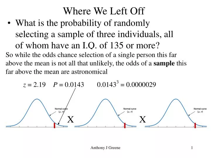
Where We Left Off. What is the probability of randomly selecting a sample of three individuals, all of whom have an I.Q. of 135 or more? Find the z -score of 135, compute the tail region and raise it to the 3 rd power.

E N D
Where We Left Off • What is the probability of randomly selecting a sample of three individuals, all of whom have an I.Q. of 135 or more? • Find the z-score of 135, compute the tail region and raise it to the 3rd power. So while the odds chance selection of a single person this far above the mean is not all that unlikely, the odds of a sample this far above the mean are astronomical z = 2.19 P = 0.0143 0.01433 = 0.0000029 X X Anthony J Greene
Sampling Distributions I What is a Sampling Distribution? A If all possible samples were drawn from a population B A distribution described with Central Tendency µM And dispersion σM ,the standard error II The Central Limit Theorem Anthony J Greene
Sampling Distributions • What you’ve done so far is to determine the position of a given single score, x, compared to all other possible x scores x Anthony J Greene
Sampling Distributions • The task now is to find the position of a group score, M, relative to all other possible sample means that could be drawn M Anthony J Greene
Sampling Distributions • The reason for this is to find the probability of a random sample having the properties you observe. M Anthony J Greene
Sampling Distributions • Any time you draw a sample from a population, the mean of the sample, M , it estimates the population mean μ, with an average error of: • We are interested in understanding the probability of drawing certain samples and we do this with our knowledge of the normal distribution applied to the distribution of samples, or Sampling Distribution • We will consider a normal distribution that consists of all possible samples of size n from a given population Anthony J Greene
Sampling Error Sampling error is the error resulting from using a sample to estimate a population characteristic. Anthony J Greene
Sampling Distribution of the Mean For a variable x and a given sample size, the distribution of the variable M (i.e., of all possible sample means) is called the sampling distribution of the mean. The sampling distribution is purely theoretical derived by the laws of probability. A given score x is part of a distribution for that variable which can be used to assess probability A given mean M is part of a sampling distribution for that variable which can be used to determine the probability of a given sample being drawn Anthony J Greene
The Basic Concept • Extreme events are unlikely -- single events • For samples, the likelihood of randomly selecting an extreme sample is more unlikely • The larger the sample size, the more unlikely it is to draw an extreme sample Anthony J Greene
The original distribution of x: 2, 4, 6, 8 Now consider all possible samples of size n = 2What is the distribution of sample means M Anthony J Greene
The Sampling Distribution For n=2Notice that it’s a normal distribution with μ = 5 Anthony J Greene
Heights of the five starting players Anthony J Greene
Possible samples and sample means for samples of size two M Anthony J Greene
Dotplot for the sampling distribution of the mean for samples of size two (n = 2) M Anthony J Greene
Possible samples and sample means for samples of size four M Anthony J Greene
Dotplot for the sampling distribution of the mean for samples of size four (n = 4) M Anthony J Greene
Sample size and sampling error illustrations for the heights of the basketball players Anthony J Greene
Dotplots for the sampling distributions of the mean for samples of sizes one, two, three, four, and five M M M M M Anthony J Greene
Sample Size and Standard Error The possible sample means cluster closer around the population mean as the sample size increases. Thus the larger the sample size, the smaller the sampling error tends to be in estimating a population mean, m, by a sample mean, M. For sampling distributions, the dispersion is called Standard Error. It works much like standard deviation. Anthony J Greene
Standard Error of M For samples of size n, the standard error of the variable x equals the standard deviation of x divided by the square root of the sample size: In other words, for each sample size, the standard error of all possible sample means equals the population standard deviation divided by the square root of the sample size. Anthony J Greene
The Effect of Sample Size on Standard ErrorThe distribution of sample means for random samples of size (a) n = 1, (b) n = 4, and (c) n = 100 obtained from a normal population with µ = 80 and σ = 20. Notice that the size of the standard error decreases as the sample size increases. Anthony J Greene
Mean of the Variable M For samples of size n, the mean of the variable M equals the mean of the variable under consideration: mM= m. In other words, for each sample size, the mean of all possible sample means equals the population mean. Anthony J Greene
The standard error of M for sample sizes one, two, three, four, and five Standard error = dispersion of MσM Anthony J Greene
The sample means for 1000 samples of four IQs. The normal curve for x is superimposed Anthony J Greene
Sampling Distribution of the Mean for a Normally Distributed Variable Suppose a variable x of a population is normally distributed with mean m and standard deviation s. Then, for samples of size n, the sampling distribution of M is also normally distributed and has mean mM = m and standard error of Anthony J Greene
(a) Normal distribution for IQs(b) Sampling distribution of the mean for n = 4(c) Sampling distribution of the mean for n = 16 Anthony J Greene
Frequency distribution for U.S. household size Anthony J Greene
Relative-frequency histogram for household size Anthony J Greene
Sample means n = 3,for 1000 samples of household sizes. Anthony J Greene
The Central Limit Theorem For a relatively large sample size, the variable M is approximately normally distributed, regardlessof the distribution of the underlying variable x. The approximation becomes better and better with increasing sample size. Anthony J Greene
M M M M M M Sampling distributions fornormal, J-shaped, uniform variable M Anthony J Greene M M M
APA Style: TablesThe mean self-consciousness scores for participants who were working in front of a video camera and those who were not (controls). Anthony J Greene
APA Style: Bar GraphsThe mean (±SE) score for treatment groups A and B. Anthony J Greene
APA Style: Line GraphsThe mean (±SE) number of mistakes made for groups A and B on each trial. Anthony J Greene
Summary • We already knew how to determine the position of an individual score in a normal distribution • Now we know how to determine the position of a sample of scores within the sampling distribution • By the Central Limit Theorem, all sampling distributions are normal with Anthony J Greene
Sample Problem 1 • Given a distribution with μ = 32 and σ = 12 what is the probability of drawing a sample of size 36 where M > 48 Does it seem likely that M is just a chance difference? Anthony J Greene
Sample Problem 2 • In a distribution with µ = 45 and σ = 45 what is the probability of drawing a sample of 25 with M >50? Anthony J Greene
z -1.96 +1.96 M 84.12 95.88 Sample problem 3 • In a distribution with µ = 90 and σ = 18, for a sample of n = 36, what sample mean M would constitute the boundary of the most extreme 5% of scores? zcrit = ± 1.96 Anthony J Greene
Sample Problem 4 • In a distribution with µ = 90 and σ = 18, what is the probability of drawing a sample whose mean M > 93? What information are we missing? n = 9 Anthony J Greene
Sample Problem 5 • In a distribution with µ = 90 and σ = 18, what is the probability of drawing a sample whose mean M > 93? n = 16 Anthony J Greene
Sample Problem 6 • In a distribution with µ = 90 and σ = 18, what is the probability of drawing a sample whose mean M > 93? n = 25 Anthony J Greene
Sample Problem 7 • In a distribution with µ = 90 and σ = 18, what is the probability of drawing a sample whose mean M > 93? n = 36 Anthony J Greene
Sample Problem 8 • In a distribution with µ = 90 and σ = 18, what is the probability of drawing a sample whose mean M > 93? n = 81 Anthony J Greene
Sample Problem 9 • In a distribution with µ = 90 and σ = 18, what is the probability of drawing a sample whose mean M > 93? n = 169 Anthony J Greene
Sample Problem 10 • In a distribution with µ = 90 and σ = 18, what is the probability of drawing a sample whose mean M > 93? n = 625 Anthony J Greene
Sample Problem 10 • In a distribution with µ = 90 and σ = 18, what is the probability of drawing a sample whose mean M > 93? n = 1 Anthony J Greene
z = ±2.58 Sample Problem 11 • In a distribution with µ = 200 and σ = 20, what sample mean M corresponds to the most extreme 1% ? n = 1 Anthony J Greene
z = ±2.58 Sample Problem 12 • In a distribution with µ = 200 and σ = 20, what sample mean M corresponds to the most extreme 1% ? n = 4 Anthony J Greene