Download
1 / 17
180 likes | 460 Views
Rolle’s theorem and Mean Value Theorem ( Section 4.2). Alex Karassev. Rolle’s Theorem. y. y. f ′ (c) = 0. y = f(x). y = f(x). f(a) = f(b). x. x. c 3. b. c 2. a. c 1. a. b. c. Example 1. Example 2. Rolles Theorem. Suppose f is a function such that f is continuous on [a,b]

E N D
Rolle’s theorem and Mean Value Theorem(Section 4.2) Alex Karassev
Rolle’s Theorem y y f ′ (c) = 0 y = f(x) y = f(x) f(a) = f(b) x x c3 b c2 a c1 a b c Example 1 Example 2
Rolles Theorem • Suppose f is a function such that • f is continuous on [a,b] • differentiable at least in (a,b) • If f(a) = f(b) then there exists at least one c in (a,b) such that f′(c) = 0 y f ′ (c) = 0 y = f(x) x a b c
Applications of Rolle’s Theorem • It is used in the prove of theMean Value Theorem • Together with the Intermediate Value Theorem, it helps to determine exact number of roots of an equation
y = cos x Example • Prove that the equation cos x = 2x has exactly one solution y = 2x
Solution • cos x = 2x has exactly one solution means two things: • It has a solution – can be proved using the IVT • It has no more than one solution – can be proved using Rolle's theorem
cos x = 2x has a solution: Proof using the IVT • cos x = 2x is equivalent to cos x – 2x = 0 • Let f(x) = cos x – 2x • f is continuous for all x, so the IVT can be used • f(0) = cos 0 – 2∙0 = 1 > 0 • f(π/2) = cos π/2 – 2 ∙π/2 = 0 – π = – π < 0 • Thus by the IVT there exists c in [0, π/2] such thatf(c) = 0, so the equation has a solution
Proof by contradiction using Rolle's theorem f(x) = cos x – 2x = 0 has no more than one solution: • Assume the opposite: the equation has at least two solutions • Then there exist two numbers a and b s.t. a ≠ b andf(a) = f(b) = 0 • In particular, f(a) = f(b) • f(x) is differentiable for all x, and hence Rolle's theorem is applicable • By Rolle's theorem, there exists c in [a,b] such that f′(c) = 0 • Find the derivative: f ′ (x) = (cos x – 2x) ′ = – sin x – 2 • So if we had f ′ (c) = 0 it would mean that –sin c – 2 = 0 orsin c = – 2, which is impossible! • Thus we obtained a contradiction • All our steps were logically correct so the fact that we obtained a contradiction means that our original assumption "the equation has at least two solutions" was wrong • Thus, the equation has no more than one solution!
f(x) = cos x – 2x = 0 has no more than one solution: visualization If it had two roots, then there would exist a ≠ b such thatf(a) = f(b) = 0 f ′ (c) = 0 y = f(x) b a c But f ′ (x) = (cos x – 2x) ′ = – sin x – 2 So if we had f ′ (c) = 0 it would mean that –sin c – 2 = 0 orsin c = – 2, which is impossible
y y y = f(x) y = f(x) x x b a b a c Example 2 Example 1 Mean Value Theorem There exists at least one point on the graphat which tangent line is parallel to the secant line
f(b) – f(a) (b-a) f′(c) = Mean Value Theorem • Slope of secant line is the slope of line through the points (a,f(a)) and (b,f(b)), so it is • Slope of tangent line is f′(c) y y = f(x) x b a c
f(b) – f(a) (b-a) f′(c) = MVT: exact statement • Suppose f is continuous on [a,b] and differentiable on (a,b) • Then there exists at least one point c in (a,b) such that y y = f(x) x b a c
Interpretation of the MVTusing rate of change • Average rate of changeis equal to the instantaneous rate of changef′(c) at some moment c • Example: suppose the cities A and B are connected by a straight road and the distance between them is 360 km. You departed from A at 1pm and arrived to B at 5:30pm. Then MVT implies that at some moment your velocity v(t) = s′(t) was:(s(5.5) – s(1)) / (5.5 – 1) = 360 / 4.5 = 80 km / h
Application of MVT • Estimation of functions • Connection between the sign of derivative and behavior of the function: if f ′ > 0 function is increasing if f ′ < 0 function is decreasing • Error bounds for Taylor polynomials
Example • Suppose that f is differentiable for all x • If f (5) = 10 and f ′ (x)≤ 3 for all x, how small can f(-1) be?
Solution • MVT: f(b) – f(a) = f ′(c) (b – a) for some c in (a,b) • Applying MVT to the interval [ –1, 5], we get: • f(5) – f(–1) = f ′(c) (5 – (– 1)) = 6 f ′(c) ≤ 6∙3 = 18 • Thus f(5) – f(-1) ≤ 18 • Therefore f(-1) ≥ f(5) – 18 = 10 – 18 = – 8