Download
1 / 15
150 likes | 293 Views
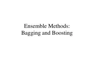
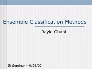
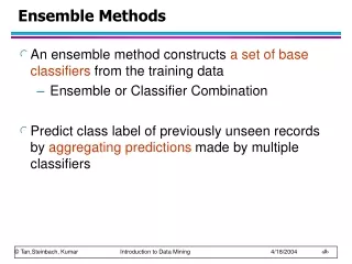
Ensemble Methods: . Bagging. Outlook. sunny. overcast. rainy. Humidity. yes. Windy. Classify the instance using the NN algorithm applied on the training instances associated with the classification nodes (leaves). high. normal. false. true.

E N D
Ensemble Methods: Bagging
Outlook sunny overcast rainy Humidity yes Windy Classify the instance using the NN algorithm applied on the training instances associated with the classification nodes (leaves). high normal false true Combining Decision Tress and the NN Algorithm
Training Data Data1 Data m Data2 Learner m Learner2 Learner1 Model1 Model2 Model m Final Model Model Combiner Ensemble Paradigm • Use m different learning styles to learn from one training data set. • Combine decisions of multiple classifiers using, e.g, weighted voting.
Why ensembles • Sometimes a learning algorithm is unstable, i.e., a little change in the training set causes a big change in the learned classifier. • Sometimes there is substantial noise in the training set. • By using an ensemble of classifiers, we don’t just depend on the decision of just one classifier. • Disadvantages • Time consuming • Over-fitting sometimes
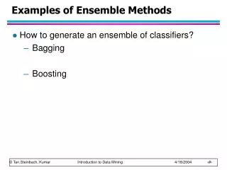
Homogenous Ensembles • Use a single, learning style but manipulate training data to make it learn multiple models. • Data1 Data2 … Data m • Learner1 = Learner2 = … = Learner m • Different methods for changing training data: • Bagging: Resample training data with replacement • Boosting: Weigh individual training vectors • In WEKA, Classify=>Choose=>classifiers=>meta They take a learning algorithm as an argument (base classifier) and create a meta-classifier.
Bag size • Original training set size: n • No. of independent base classifiers: m • For each base classifier, randomly drawing n’ examples from the original data, with replacement • n’ usually < n • If n=n’, on average it will contain 63.2% unique training examples. The rest are duplicates. • Combine the m resulting models using simple majority vote. • Decreases overall error by decreasing the variance in the results due to unstable learners, algorithms (like decision trees) whose output can change dramatically when the training data is slightly changed.
Satellite Images Data • http://archive.ics.uci.edu/ml/datasets/Statlog+(Landsat+Satellite) • Generated by NASA • Own by the Australian Centre for Remote Sensing • One frame of Landsat imagery consists of 4 digital images of the same scene in 4 different spectral (wavelength) bands. • Two of these are in the visible region: green and red • Two are in the near infra-red • A pixel in the image corresponds to 80m by 80m of real land • Pixel value = spectral band intensity • Pixel value = 0 means darkest • Pixel value = 255 means brightest
Record format • Example: 92 115 120 94 84 102 106 79 84 102 102 83 101 126 133 103 92 112 118 85 84 103 104 81 102 126 134 104 88 121 128 100 84 107 113 87 3 • Each line of data corresponds to a 3x3 square neighborhood of pixels • Example:921151209484102106798410210283101126133103921121188584103104811021261341048812112810084107113873 • Each line contains the pixel values in the 4 spectral bands • (3x3)x4 = 36 numbers • The last number indicates type of land • The records are given in random order so that you cannot reconstruct the original landscape
Class labels There are no examples with class 6 in this particular dataset. The classification for each pixel was performed on the basis of an actual site visit by Ms. Karen Hall, when working for Professor John A. Richards, at the Centre for emote Sensing at the University of New South Wales, Australia.
Weka’s bagging • Single classifier • Use satellite image training and test data • Classify test data using NaiveBayesSimple • Observe the outputs • Bagging • Classify=>Choose=>meta=>Bagging • Set bagSizePercent to 80 • Try numIterations = 80 • Observe error rate • Try numIterations = 90 • Observe error rate
Misclassification rates • CART: Classification And Regression Tree


![[[PDF]] Ensemble Learning: Pattern Classification Using Ensemble Methods (Second Edition) BY-Lior Rokach](https://cdn5.slideserve.com/10147553/slide1-dt.jpg)