Download
1 / 54
630 likes | 1.02k Views
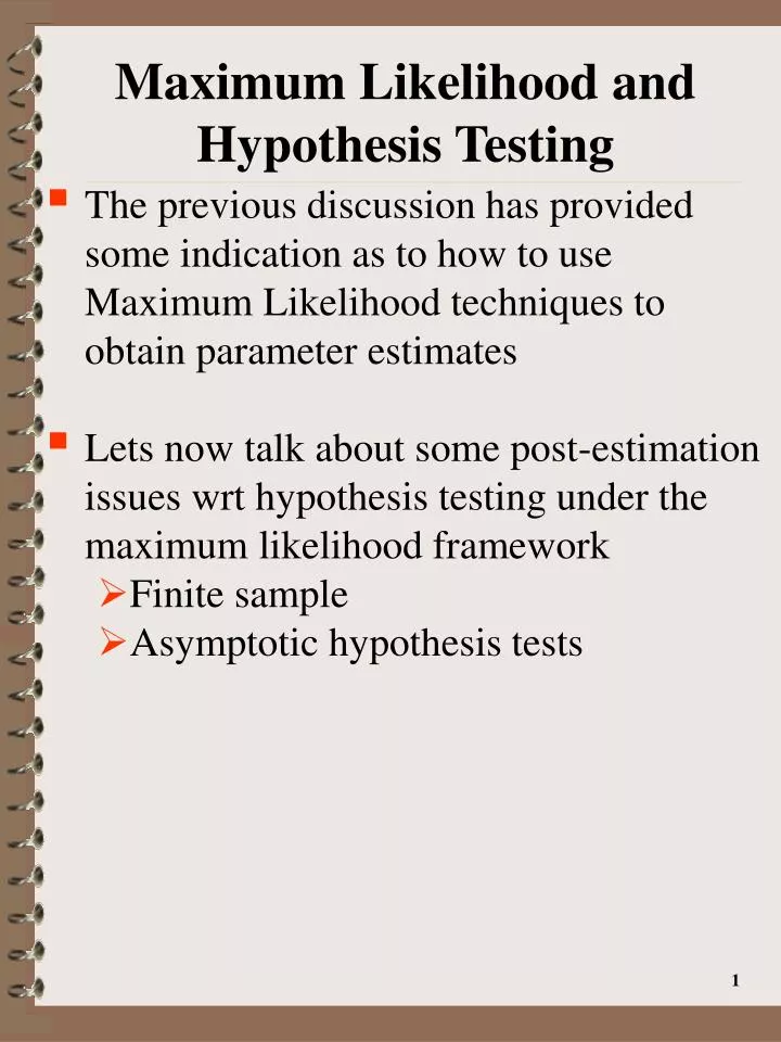
Maximum Likelihood and Hypothesis Testing. The previous discussion has provided some indication as to how to use Maximum Likelihood techniques to obtain parameter estimates Lets now talk about some post-estimation issues wrt hypothesis testing under the maximum likelihood framework

E N D
Maximum Likelihood and Hypothesis Testing • The previous discussion has provided some indication as to how to use Maximum Likelihood techniques to obtain parameter estimates • Lets now talk about some post-estimation issues wrt hypothesis testing under the maximum likelihood framework • Finite sample • Asymptotic hypothesis tests
Maximum Likelihood and Hypothesis Testing • As we discussed earlier, a standard test procedure is based on relative likelihood function values under a null hypothesis(s) versus its value unrestricted • Likelihood Ratio Test (finite sample): Compare sample likelihood function value, l(•), under the assumption that the null hypothesis(s) is true, [l(Ω0)] vs. its value with unrestricted parameter choice [l*(Ω)] • Null hypothesis(s) (H0) could reduce the allowable set of parameter values. • What does this do to the maximum likelihood function value? • If the two resulting maximum likelihood function values are close enough → can not reject H0
Maximum Likelihood and Hypothesis Testing • Is this difference in likelihood function values large? • Likelihood ratio (λ): • λ is a random variable since l(·)’s depend on yi’s which are R.V.’s • What are possible values of λ? • l(Ω0)≤ l*(Ω) → λ≥1 unrestricted l(·) restricted l(·)
Maximum Likelihood and Hypothesis Testing • Likelihood Ratio (LR) Principle • Null hypothesis defining Ω0 is rejected if λ > 1 • Need to establish critical level of λ, λC,that is unlikely to occur under H0 (e.g., is 1.1 far enough away from 1.0 given that λ is a RV)? • Reject H0 if estimated value of λ > λC • λ = 1→Null hypothesis(s) does not significantly reduce parameter space • H0 not rejected • Result conditionalon sample
Maximum Likelihood and Hypothesis Testing • General Likelihood Ratio (LR) Test Procedure • Choose probability of Type I error, a (e.g., test significance level) • Given a, find value of lC that satisfies: P(l >lC | H0 is true) = α • Evaluate test statistic based on sample information • Reject (fail to reject) null hypothesis if l >lC (< lC)
Maximum Likelihood and Hypothesis Testing y~N(μ, σ2) • LR test of the mean of Normal Distribution (µ) with s2not known • This implies the following test procedures given LR* and assuming a normally distributed RV and testing for the mean, • F-Test • t-Test • LR test of hypothesized value of s2 variance of mean Note: Finite sample tests given linear model
Maximum Likelihood and Asymptotic Hypothesis Tests • Previous tests based on finite samples • Use asymptotic tests when appropriate finite sample test statistic is unavailable • These rely on Central Limit Theorem and asymptotic normality of ML estimators • For example when have models where the functional form is nonlinear in parameters • Three asymptotic tests commonly used: • Asymptotic Likelihood Ratio Test • Wald Test • Lagrangian Multiplier (Score) Test • For a review: • Greene: 524-534, JHGLL: 105-110. • Buse article(on website)
Maximum Likelihood and Asymptotic Hypothesis Tests • Lets start simple where we have a single parameter, θ • Assume you want to • Undertake ML estimation of θ • Test of the hypothesis, H0: c(θ)=0 • The logic of the three asymptotic tests procedures can be obtained from the following figure • Plots for alternative values of θ: • The sample log-likelihood function, L(θ) • The gradient of the sample log-likelihood function, dL(θ)/dθ • The value of the function, c(θ)
Maximum Likelihood and Asymptotic Hypothesis Tests L(θ), dL(θ)/dθ, c(θ) .5* Likelihood Ratio dL(θ)/dθ L(θ) L H0: c(θ)=0 LR c(θ) Lagrangian Multiplier Wald θ θML θML,R Greene, p. 499
Maximum Likelihood and Asymptotic Hypothesis Tests H0: c(θ)=0 • Summary of Asymptotic Hypothesis Tests • Asymptotic Likelihood Ratio Test: If c(θ) is valid, them imposing it should not impact L(θ) significantly. • → base test on difference in L(θ)’s across the two points θML and θML,R • Wald Test: If c(θ) is valid, then c(θML) should be close to 0 • → base test on θMLandc(θML) • reject H0 if c(θML) is significantly different from 0 • Lagrange Multiplier Test: If c(θ) is valid, then θML,R should be near the point the maximizes LF • → slope of LF should be close to 0 • base test on slope of LLF at θML,R
Maximum Likelihood and Asymptotic Hypothesis Tests • These three tests are asymptotically equivalent under H0 • They can behave differently in a small samples • Small sample properties are typically unknown • → Choice among them is typically made on basis of computational ease • LR test requires calculation of both restricted and unrestricted estimates of parameter vector • Wald tests requires only unrestricted estimate of parameter vector • LM test requires only restricted estimate of parameter vector
Maximum Likelihood and Asymptotic Hypothesis Tests • Let y1,…,yT be a set of RVs w/joint PDF: fT(y1,…,yT| ) where is a (K x 1) vector of unknown parameters where Ω(allowable parameter space) • The sample likelihood and log-likelihood functions given our data are: • l(|y1…yT) • L(|y1…yT) ≡ lnl(|y1…yT) • As sample size, T, becomes larger, lets consider testing the hypotheses: R()=[R1(),R2(),…,RJ()]' → Ω0 allowable parameter space under the J hypotheses
Maximum Likelihood and Asymptotic Hypothesis Tests • Likelihood Ratio • λ ≡ l*(Ω)/l(Ω0) or l(ML)/l(0) • l*(Ω) = Max[l(|y1,…,yT):Ω] • Unrestrictedlikelihood function • l(Ω0) = Max[l(|y1,…,yT):Ω0] • Restricted likelihood function assuming null hypothesis is true • Asymptotic Likelihood Ratio (LR) • LR ≡ 2ln(λ) = 2[L*()-L(0)] • L(·) ≡lnl(·) • What is the sign of LR? • LR~χJ asymptotically where J is the number of joint null hypothesis (restrictions) • Theorem 16.5, Greene p.500
Maximum Likelihood and Asymptotic Hypothesis Tests Asymptotic Likelihood Ratio Test H0: Ω0 0 l L(l) L() .5LR L(0) L≡ Log-Likelihood Function LR ≡ 2ln(l)=2[L(1)-L(0)] LR~c2(α,J) asymptotically (p.105 JHGLL) Evaluated L(•) at both 1 and 0 L l generates unrestricted L(•) max L(0) value obtained under H0
Maximum Likelihood and Asymptotic Hypothesis Tests • Greene defines the above as: -2[L(0)-L*()] • Result is the same • Buse, p.153, Greene p.498-500 • As noted above, given H0 true, LR has an approximate χ2 dist. with J DF • Reject H0when LR > χc where χc is the predefined critical value of the distribution given J DF and desired Pr(Type I error). • In MATLAB we can generate the critical χ2 value of H0 testing • critical_valu • = chi2inv(1-p_type_1,num_rest) • p_type_1 is Pr(Type I error)
Maximum Likelihood and Asymptotic Hypothesis Tests • Example of an inappropriate use of the likelihood ratio • Use the LR to test one distributional assumption against another (e.g., normal vs. logistic) • The parameter spaces and therefore likelihood functions are unrelated • To be appropriate, the restricted model needs to be nested within the original likelihood function • → alternative model obtained from original model via parameter restrictions only not a change in functional form as in the above normal vs. logistic example
Maximum Likelihood and Asymptotic Hypothesis Tests • Asymptotic Likelihood Ratio (LR) • LR ≡ 2ln(λ) = 2[L*()-L(0)] • L(·) ≡lnl(·) • L*() ≡ Unrestricted LLF • L() ≡ Restricted LLF subject to c(Θ) =0 • LR ~ χJ asymptotically • J is the number of joint null hypothesis (restrictions)
Maximum Likelihood and Asymptotic Hypothesis Tests • A size corrected asymptotic Likelihood Ratio statistic • In our estimation of the error term variance we often use a correction factor that accounts for the number of parameters used in estimation • Improved the approx. to the sampling distribution of the statistic generated from its limiting χ2 distribution • A similar correction factor has been suggested by Mizon (1977, p.1237)) and by Evans and Savin (1982, p.742) to be applied to the asymptotic LR • These size-correction factors have been applied to the asymptotic LR to improve its small sample properties
Maximum Likelihood and Asymptotic Hypothesis Tests • Mizon’s (1977) size corrected LR statistic: K = Number of explanatory variables including intercept term J = the number of joint hypotheses LR = the traditionally calculated log- likelihood ratio • = 2[L*()-L(0)]
Maximum Likelihood and Asymptotic Hypothesis Tests • Lets provide a motivation for the Asymptotic Wald test • Suppose consists of 1 element • H0: Θ = Θ0 or Θ–Θ0= 0 • 2 samples • Generate different LF estimates • Same value maximizes the LF’s
Maximum Likelihood and Asymptotic Hypothesis Tests 0 l Max at same point L(l) .5LR0 L() L(0) .5LR1 L1(0) L1() H0: =0 Two samples L • 0.5LR will depend on two factors: • Distance between l and 0(+) • The curvature of the LF (+) 21
Maximum Likelihood and Asymptotic Hypothesis Tests Impact of Curvature on LR Shows Need For Wald Test • 0.5LR will depend on • Distance between l and 0(+) • The curvature of the LF (+) • V() represents LF curvature • Wald Test based on the following statistic given the H0: Θ = Θ0 • W=(l-0)2 V(|=l)-1 Single Parameter assuming concavity Don’t forget the “–” sign
Maximum Likelihood and Asymptotic Hypothesis Tests Impact of Curvature on LR Shows Need For Wald Test 0 l Max at same point L(l) .5LR0 L() L(0) L1() .5LR1 L1(0) Two samples H0: = 0 W=(l-0)2 V(|=l)-1 W~c2J asymptotically Note: Evaluated atl unrestriced value L
Maximum Likelihood and Asymptotic Hypothesis Tests • Wald statistic: weights squared distance, (l - 0)2 by the curvature of LF instead of using the differences in LF values as in LR test • Two sets of data may produce the same (l - 0)2 value but give different LR values because of curvature • The more curvature, the more likely H0 not true (e.g., test statistic is larger) • Greene, p. 500-502 gives alternative motivation, Buse, p. 153-154 H0: Θ = Θ0
Maximum Likelihood and Asymptotic Hypothesis Tests • The asymptotic covariance matrix of the ML estimator is based on the Information Matrix of estimated parameters • If the form of the expected values of the 2nd derivatives of the LLF are known: • A 2nd estimator is: • A 3rd estimator is: Measure of curvature 25
Maximum Likelihood and Asymptotic Hypothesis Tests Let c(Θ) represent J joint hypotheses • Extending to J simultaneous hypotheses, K parameters and more complex H0’s: q is target Can use any of the 3 methods • Note that c(∙), d(∙) and I(∙) evaluated at ML, the unrestricted value • When cj(q) of the form: j=j0, j=1,…K • d()=IK, • W=(l-0)2 I(|=l) (K x K) identity matrix
Maximum Likelihood and Asymptotic Hypothesis Tests • In summary, Theorem 16.6, Greene p.501: With the set of hypotheses represented by H0: c(θ) = q, the Wald statistic is: d(θML)I(θML)-1 d(θML)′
Maximum Likelihood and Asymptotic Hypothesis Tests • The Wald test is based on measuring the extent to which the unrestricted estimates fail to satisfy the hypothesized restrictions • Large values of W→ large deviations of c(Θ) away from q are weighted by a matrix involving curvature of the log-likelihood function • Shortcomings of the Wald test • It is a pure significance test against the null hypothesis not necessarily for a specific alternate hypothesis • The test statistic is not invariant to the formulation of the restrictions • Test of a function θ=β/(1-γ) equals a specific value q.
Maximum Likelihood and Asymptotic Hypothesis Tests θ≡β/(1-γ) = q? • Two ways to evaluate this expression • Determine variance of the non-linear function of β and γ • β-q(1-γ) = 0 which is equivalent but a linear restriction based on the two parameters, β and γ. • The Wald statistics for these two tests could be different and might lead to different inferences
Maximum Likelihood and Asymptotic Hypothesis Tests Summary of Lagrange Multiplier (Score) Test • Based on the curvature of the log-likelihood function [L(Θ)] but this time at therestricted log-likelihood function value • At unrestricted maximum: Score of Likelihood Function
Maximum Likelihood and Asymptotic Hypothesis Tests S() ≡ dL/d 0 Θ0 clser to optimum under sample B L(0) S()=0 S(0) Two samples H0: Θ = Θ0 LA LB L • Sample B has the greater curvature of L(∙) when evaluated at 0 • Both samples have the same gradient at Θ0, the hypothesize value
Maximum Likelihood and Asymptotic Hypothesis Tests Summary of Lagrange Multiplier (Score) Test • How much does S() depart from 0 when evaluated at the hypothesized value? • Weight squared slope (to get rid of negative sign) by curvature • The greater the curvature, the closer 0will be to the maximum value • Weight by V()→smaller test statistic the more curvature in contrast to Wald test Single Parameter In contrast to Wald which uses V(Θ)-1
Maximum Likelihood and Asymptotic Hypothesis Tests Summary of Lagrange Multiplier (Score) Test • How much does S() depart from 0 when evaluated at the hypothesized value? • Small values of test statistic, LM, will be generated if the value of L(0) is close to the maximum value, L(l), e.g. slope closeto 0 33
Maximum Likelihood and Asymptotic Hypothesis Tests • When comparing samples A and B: • Sample B→ smaller test statistic because 0 is nearer max. of its log-likelihood (e.g. S(0) closer to zero) S() ≡ dL/d 0 L(0) S()=0 S(0) Two samples LA LB L
Maximum Likelihood and Asymptotic Hypothesis Tests • Suppose we maximize the log-likelihood subject to the set of constraints, c(Θ)-q = 0 • λ is the set of Lagrangian multipliers associated with the J-constraints (hypotheses) • Solution to constrained maximization problem must satisfy the following two sets of FOC’s:
Maximum Likelihood and Asymptotic Hypothesis Tests • If the restrictions are valid, then imposing them will not lead to a significant difference in maximized value of the LF • i.e., L*(Θ)|Θ=Θ0 ≈ L(Θ)|Θ=Θ0 • → second term in the 1stfirst-order condition,d(Θ)′λ, will be small • Specifically, λ will be small given d(Θ) is the derivative of c(Θ) whose value will probably not be small • We could directly test if λ=0 This should be close to zero if null hypothesis is true
Maximum Likelihood and Asymptotic Hypothesis Tests H0: Θ = Θ0 • Alternatively, at the restricted maximum, from (1) the derivatives of the LF are: • If hypotheses are in fact true then • gR= 0 • → the derivatives of the unrestricted LLF, L(Θ) evaluated at Θ0 ≈ 0 37
Maximum Likelihood and Asymptotic Hypothesis Tests Derivative of original LLF but at the restricted values • The above implies we need to determine whether the K slopes are jointly zero • Evaluate slopes at restricted values • The variance of the gradient vector of L(Θ) is the information matrix, I(Θ), which has been used in the evaluation of the parameter covariance matrix • The above is property P.3 of the L(Θ) stated in my introductory ML comments (Greene, p.488) • Need to evaluate I(Θ) matrix at the restricted parameter vector • I(Θ)|Θ = Θ0 = negative of the expected value of the LLF Hessian matrix at Θ = Θ0
Maximum Likelihood and Asymptotic Hypothesis Tests Summary of Lagrange Multiplier (Score) Test S() ≡ dL/d 0 Gradient vector (of L(Θ)) variance is I(Θ) L(0) S()=0 S(0) Two samples LA LB L LM= S(0)2 I(0)-1 S(0)=dL/d|=0 I(0) = -d2E(L/d2|=0) LM~c2J asympt. Restricted values
Maximum Likelihood and Asymptotic Hypothesis Tests • Extending to multiple parameters S(Θ) ≡ dL/dΘ, Var(S(ΘML)) = −E(HML) = I(Θ) [Theorem 16.2 Greene p. 488] • Theorem 16.7, Greene p. 503 provides LM statistic • Buse, pp. 154-155
Maximum Likelihood and Asymptotic Hypothesis Tests • LR, W, LM differ in type of information required • LR requires both restricted and unrestricted parameter estimates (e.g., evaluate LF twice) • Wrequires only unrestricted estimates • LMrequires only restricted estimates • If log-likelihood is quadratic with respect to Θ, the 3 tests result in same numerical values for large samples
Maximum Likelihood and Asymptotic Hypothesis Tests • All test statistics distributed asymptotic c2 with J d.f. (number of joint hypotheses) • Theoretically, in finite samples W≥LR≥LM • →LM more conservative in the sense of rejecting H0 less often • Lets revisit the previous example where we examined the relationship between income and educational attainment • Greene, p. 531 • Previously we examined the following conditional exponential distribution:
Maximum Likelihood and Asymptotic Hypothesis Tests • Greene, p.531 extends the exponential density to a more general gamma distribution where the exponential is nested • To save on notation, define the following: • The general gamma distribution can be represented via the following: ρ additional parameter gamma function
Maximum Likelihood and Asymptotic Hypothesis Tests • Given the above sample log-likelihood we have the following derivatives (Greene, p. 531): • Note: I do not use these in estimation but in post-estimation evaluation of Hessians and hypothesis testing 44
Maximum Likelihood and Asymptotic Hypothesis Tests Gamma dist. • When ρ=1 → Γ(ρ)=1 • →Exponential distribution is nested within the above general distribution • We can test the null hypothesis that the distribution of income is exponential versus gamma wrt educational attainment • H0: ρ = 1 H1: ρ ≠ 1 Exponential dist. 45
Maximum Likelihood and Asymptotic Hypothesis Tests Gamma dist. • The total sample log-likelihood for the general gamma distribution is: • As before the total sample log-likelihood for the exponential distribution is
Maximum Likelihood and Asymptotic Hypothesis Tests • The following MATLAB code is used to estimate the β and ρparameters • Unrestricted parameter estimates implicitly obtained by setting first derivatives equal to 0 • Restricted parameter estimates by setting ρ=1 and ∂L(β|ρ=1)/∂β=0 • Three estimates of parameter covariance matrix are obtained • NR (Hessian-based) ΣNR=[-∂2L/∂ΘΘ′]-1 • GN (Expected Hessian-based) ΣGN=[-E(∂2L/∂ΘΘ′)]-1 where E(Inci|Edui)=ρ(β+Edui) • BHHH (Sum Sq. and Cross Prod.) ΣBH=[Σi(∂Li/∂Θ) (∂Li/∂Θ)′]-1 Estimation Method
Maximum Likelihood and Asymptotic Hypothesis Tests 48
Maximum Likelihood and Asymptotic Hypothesis Tests Gamma dist. • The total sample log-likelihood for the general gamma distribution is: • As before the total sample log-likelihood for the exponential distribution is
Maximum Likelihood and Asymptotic Hypothesis Tests • Lets test whether the distribution is gamma or exponential • H0: ρ=1 (exponential) H1: ρ≠1 • Confidence Interval: 95% CI based on unrestricted parameter results • Likelihood Ratio Test: • λ=2[– 82.9144 – (–88.4377)]=11.046 • 1 DF, critical value is 3.842 restricted LLF Unrestricted LLF