Download
1 / 27
280 likes | 411 Views
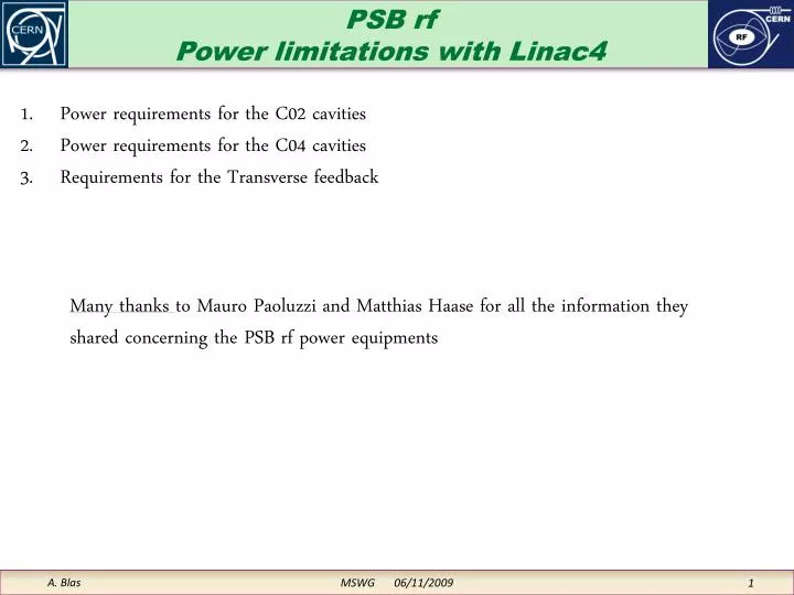
Power requirements for the C02 cavities Power requirements for the C04 cavities Requirements for the Transverse feedback. PSB rf Power limitations with Linac4. Many thanks to Mauro Paoluzzi and Matthias Haase for all the information they shared concerning the PSB rf power equipments.

E N D
Power requirements for the C02 cavities Power requirements for the C04 cavities Requirements for the Transverse feedback PSB rfPower limitations with Linac4 Many thanks to Mauro Paoluzzi and Matthias Haase for all the information they shared concerning the PSB rf power equipments MSWG 06/11/2009
The cavity amplifier needs to supply the current necessary to: Create the required voltage into the bare cavity => I0 Provide the accelerating energy => IA … and also compensate the effect of loop errors => IP Beam loading in cavities MSWG 06/11/2009
Currents within a cavity I0 corresponds to the current IG when there is no beam and a perfectly tuned cavity. I0 also corresponds to the current requirement with any beam intensity when the tuning error and the stable phase are null (coasting beam). For 8 kV on C02, I0 = 3 Apeak For 8 kV on C04, I0 = 1 Apeak During acceleration, the extra current to be supplied by the amplifier is > IB * sin (ΦB) MSWG 06/11/2009
Sine shape approximation Beam current φL , TL For a pure h1 or h2 beam, the beam peak current is 22.7 A @ ej 1st rf harmonic : ÎH1 = 9.56 A 2nd rf harmonic: ÎH2 = 6.06 A w/o acceleration, the h1 bunch length: φL 138o (2.4 rad or 220 nsh1 @ej.) Total charges per bunch= 2 E13h1 (sinus shape approx.) MSWG 06/11/2009
Fourier components Phases and harmonics are declared with respect to the rf Sine shape approximation Beam current φL , TL During the acceleration φL [rf rad] remains almost constant when accelerating with a single harmonic => The beam current harmonics amplitude is typically proportional to FREV only for a given beam charge and a single harmonic acceleration (constant bunch length). MSWG 06/11/2009
We have seen that the “accelerating” current from the amplifier is: IA > IB sin(ΦB) For a single particle or a short bunch, ΦB and φS are identical, but when the bunch is wider, its 1st harmonic phase changes due to the asymmetry of the accelerating bunch. When the bunch is longer, the first harmonic amplitude get smaller => ΦB is increasing to supply the same accelerating energy. All in all, for the same beam charge, the “accelerating” should remain the same. Current required from the amplifierfor the acceleration It can be shown that: For R=25m, ρ=8.24m and VRF = 8000V: In the present cycles with Bdot max = 2.2 T/s: sinφS = 0.35 and φS=20.6o (rf angle) The maximum current required from the power amplifier is: For 2.1013p and φL = 2.4: This expression is valid for both a pure h1 or h2 acceleration MSWG 06/11/2009
In the present 50 MeV to 1.4 GeV cycle, the highest IA is required around C615 where Bdot = 2.2 T/s and FREV = 1.645 MHz Current required from the amplifierfor the acceleration • For a cavity to accelerate the beam in a single harmonic mode requires: • IA max > 3.22 A = 0.89 * 1.645 * 2.2, not including the tuning phase errors effect. MSWG 06/11/2009
CO2 The C02 (h1) cavity tetrode can supply 24 Apeak which corresponds to 6 Apeak at the Gap. 3 A at the gap are required to provide the nominal 8 kV…in a ideal steady state situation (no error, no-acceleration). => 3 A are available in C02 to accelerate the beam and compensate for possible tuning loop errors. The tuning loop bandwidth is in the order of 500 Hz. Current capabilities of the amplifiers => The C02 amplifier doesn’t fulfill the requirements (3 A < 3.22 A), for a pure h1 acceleration with the present magnetic cycle. MSWG 06/11/2009
CO4 The C04 (h2) cavity tetrode-pair can supply 7 Apeak which corresponds to 3.5 Apeak at the Gap. 1A is required in a ideal steady state situation (no tuning error, no-acceleration). This leaves us with a 2.5 A overhead that can be used to accelerate the beam and compensate for possible tuning loop errors. The tuning loop bandwidth is in the order of 4 kHz. Current capabilities of the amplifiers => The C04 amplifier doesn’t fulfill the requirements (2.5 A < 3.22 A) for a pure h2 acceleration with the present magnetic cycle. MSWG 06/11/2009
Lower the maximum Bdot • For an h1 acceleration, the current demand on C02 should go down to 3 A instead of 3.22 A • This means a maximum Bdot reduced by factor 3.22/3. • Bdot < 2.05 T/s (2.2 T/s presently) • For an h2 acceleration, the current demand on C04 should go down to 2.5 A instead of 3.22 A • This means a maximum Bdot reduced by factor 3.22/2.5. • Bdot < 1.7 T/s (2.2 T/s presently) • Without lengthening the present cycle, B dot could be decreased thanks to the increased injection energy. • The present 50 MeV -> 1.4 GeV acceleration lasts 490 ms (C275, 1251 G -> C765, 8610 G) • From 50 MeV to 160 MeV, the acceleration lasts 123 ms (C275, 1251 G -> C398, 2300 G) • Considering that for the same Bdot, the cycle could be 60 ms (=123 ms/2)?) shorter, keeping the same cycle duration could mean 12% (60 ms/490 ms) less Bdot. • We could get Bdot = 1.96 T/s at no cost (?) How to reduce the current demand ? MSWG 06/11/2009
Lower the maximum Bdot The accelerating period could be lengthened by making the extraction flat-top shorter. The new beam control is (should be) capable of outputting a synchronized beam at the very start of the flat-top. The flat-top is 40 ms long, reducing it to 5 ms (is this compatible with the settling of the dipolar power supplies?) would allow 35 ms more for the acceleration. Together with the equivalent 60 ms obtained from the highest injection energy, there is possibly an equivalent 95 ms or 19% gain for the acceleration duration. 2.2 T/s /1.19 = 1.85 T/s > 1.7 T/s How to reduce the current demand ? MSWG 06/11/2009
The re-arrangement of the accelerating cycle leading to a Bdot reduced to 1.85 T/s should be enough to allow for a full beam acceleration with the present C02 setup. We still need to make a measurement campaign to estimate the tuning errors. These tuning errors might be reduced by the smoother behavior of the future beam control with optimized loop filters. 1.85 T/s is superior to the 1.7 T/s limit of the C04 cavity in case of a pure h2 acceleration. This doesn’t seem important as the top intensity is not expected to be accelerated in a single h2 mode. C04 is also limited in its maximum power dissipation (air cooling), this aspect still needs to be further investigated. The power limits can be tested by creating a cycle with a higher Bdot(x 2 = 4.4 T/s) Summary of the power requirements MSWG 06/11/2009
In the rf context, beam loading refers to the beam current to the cavity real current (typically the amplifier current) ratio = IB/I0. This ratio appears as limiting factor of the stability domain of the overall rf setup. Beam loading in the PSB cavities Block diagram of the different loops involved in the Pedersen’s model Simplified Pedersen’s stability criteria in the context of short bunches, B = 0, L =0 and S small compared to cavity bandwidth. A,T,P are resp. the Amplitude, Tuner, Phase loop gain Pedersen’s model describing the beam control interactions taking into account the phase-amplitude coupling of linear system driven by modulated signals. MSWG 06/11/2009
The Pedersen’s model takes into account the fundamental modes in a single harmonic context. An analytical stability criteria was found only in simplified contexts (short bunches, small synchrotron frequency, no acceleration, no tuning error, large cavity BW) The model describing an overall dual harmonic system is likely to be very complicated. No one (that I know of) did the exercise. Anyhow, even the analysis made on a single harmonic depicts the problem without giving a real cure. What appears, is that increasing the cavity bandwidth lowers the amplitude-phase interaction and its resulting stability domain reduction. So, up to now, the method used to improve the situation has been to reduce the cavity impedance (increased bandwidth perceived by the beam) by means like the wideband feedback and the 1TFB (not installed in the PSB). Increasing the RF voltage is also a way to deal with it, as long as the amplifier permits it, and as long as the beam current doesn’t increase to much due to the bunch shortening. Beam loading in the PSB cavities MSWG 06/11/2009
What new can be done? In the context of a fully digital beam control where all the low-level transfer functions are well defined, a truthful model can be simulated. Although there is little hope to see arise an analytical criteria for stability, some beneficial changes may be found empirically !? More is expected from a cartesian (or I/Q) loop system (as opposed to the present polar loop). In a system where the modulated signals are not decomposed into phase and amplitude as it is the case in the PSB, but remain described as a vector with I/Q coordinates, the interactions are different. From coffee discussions with my LHC colleagues, using this kind of feedback is without a doubt the solution…. but there is no proof either(?) Anyone heard about some analysis being done (?) The AVC and Tuner loops need to be integrated into the low-level system. First it allows for a precise definition and setting of the feedback paths, but also allows implementing the I/Q loops like in LEIR (no tuner loop on this machine). In mid-April 2009 took place a meeting with Mauro, in charge of the PSB power system. He agreed on shifting the responsibility of the AVC and Tuner loop to the low-level crew. Some security issues need first to be assessed (work in progress) Beam loading in the PSB cavities MSWG 06/11/2009
Example of I/Q AVC loopThe Leir system MSWG 06/11/2009
In 2007 some MD’s have been carried-out to evaluate the stability threshold of the C04 cavity on the extraction plateau. In this experiment, the voltage of the second harmonic cavity (C04) has been lowered on a dual harmonic high intensity beam (lowering of I0 and as the bunch gets shorter, increase of IB) until the beam gets unstable. This operation (lowering of the h2 voltage) is classically required to match longitudinally PS and PSB. The result of the MD was that below VH2 = 1.67 kV (with VH1 = 8 kV), instabilities occur with 8E12 charges (IB h2 = 2.42 A). A tempting extrapolation is to foresee a minimal VH2 = 1.67 x 2 / 0.8 = 4.17 kV with 2E13 p This approach is conservative as the beam signal drops when the h2 voltage is increased (cumulative effect) Testing the limits ofbeam loading instabilities VH2 > 4 kV at the highest L4 intensity (effect on PS matching?) If the C02 cavity is assumed to react the same way as C04 concerning the beam loading, the lower voltage threshold with 9.56A (2E13 p) would be 1.67*9.56/2.42 = 6.6 kV < 8kV MSWG 06/11/2009
The C02 should be able to cope with the 2E13 p beam As long as the cycle remains as long as it is! The C04 will (just) not be able to accelerate the full intensity on h2 with the present cycle length. Summary of the cavitiesPower issues It should nevertheless be capable of doing all what is required for bunch shaping VH2 > 4 kV at extraction for the highest intensity (H1+H2 context) Solution: I/Q loop ? Thermal issues are still to be assessed (on C04 especially) !? Tests can be achieved Use higher Bdot to simulate the effect of a higher beam current, make beam shorter to create beam loading on C02 MSWG 06/11/2009
The present transverse feedback is “marginally” well dimensioned to keep all operational beams stable up to the maximum intensity ( 1013 charges per Ring). Losses are sometimes encountered at a maximum Beam intensity on the extraction plateau, most often on Ring 4 and rarely on Ring 1. These losses may be avoided by a fine setting of the synchronization loop and machine tune. Power issuesin the PSB Transverse Feedback MSWG 06/11/2009
Present system Power issuesin the PSB Transverse Feedback • Two 100W amplifiers drive in Push-Pull opposite strip-line plates in the ring. • Vertical Plane not used, except for MDs • Although the system has been designed for a total bandwidth of 100 MHz, it is now covering a limited BW of 13 MHz. This was found to be sufficient and eases the setting-up of the system (less sensitive to loop delay errors). • With 200 W in the horizontal plane only, the system is well dimensioned for 1013 charges (just!) • Ageing low level system MSWG 06/11/2009
Future system • If the parasitic field created by the beam current is proportional to the intensity, a doubling of the intensity means a doubling of the parasitic Field • A Doubling of the exciting field implies a doubling of the damping field • Doubling the kicker voltage mean multiplying by 4 the drive power • 400W amplifiers (and final matching resistors) instead of the present 100 W units would be marginally adequate. Power issuesin the PSB Transverse Feedback There might be hidden impedances that can create instabilities with a higher intensity How can we spot these impedances to adapt the bandwidth accordingly? MSWG 06/11/2009
GLOBAL STRATEGY (not proved to be correct yet): Use a low power TFB system but with the widest possible bandwidth (the PSB transverse feedback is capable of 100 MHz by removing a low-pass filter) Increase the gain of the betatron excitation by making the TFB loop marginally (un)stable. This is achieved by: 1) inverting the loop phase 2) setting the loop gain just below instability 3) setting the Q value in order to have an open loop transfer function real (and negative) at the very betatron line (presently in the PSB, there is no Betatron phase setting within the loop) Track the hiddenTransverse impedances |CLTF|=|G/(1+GH)| OLTF = G.H Im IN Σ G OUT ω -1 Re H Freq. ω MSWG 06/11/2009
At which frequency is the resonant impedance? This question is of interest to establish the required bandwidth and also to localize by deduction the faulty element in the ring. and also to get an idea of its actual impedance in Ohms (used as a calibration when searching for new impedances; see following slides). Proposed setup: The beam is accelerated without TFB at the lowest intensity where we just start noticing a transverse excitation. At this very limit (not inducing losses) the beam is just tickling the top of the impedance (the centre of the resonance). If we do a FFT along these instants we see the emergence of betatron lines Track the hiddenTransverse impedances Rev lines Betatron lines f [Hz] Candidates MSWG 06/11/2009
If you repeat the same procedure with another tune value, you get a second set of different candidates. Compare then the 2 sets of frequency candidates: if not only one does coincide within the precision of the measurement => make another measurements until you find only one frequency value that is common to all measurements. (one half of the lines can be disregarded as they are naturally stable) If you still have to many applicants, check which mode is excited (analysis of the time signal) to evaluate which frequency line is more likely to be selected. Track the hiddenTransverse impedances Rev lines Betatron lines f [Hz] Candidates MSWG 06/11/2009
In an accelerating cycle you might have difficulties to precisely spot the start of the excitation in terms of frequency value. The FFT take longer if you need resolution and the longer, the more frequency averaging due to the acceleration. There is a tradeoff value to be found for the FFT. To avoid this difficulty, use a frequency plateau, if possible, and change the tune until you cross the resonance. This was tried in the PSB on a 160 MeV Flat cycle. Another possibility to consider is that the impedance may be of a comb type (ex: non terminated line). This can be taken into account as a criteria in the frequency line selection. … you may also have many different narrow band impedances in the ring (meaning possibly that you should give up ) Track the hiddenTransverse impedances MSWG 06/11/2009
This method has been used to highlight a transverse resonance at 1,66 MHz. Corresponds to the impedance of the extraction kicker as simulated by M. Chanel with C. Carli’s software. Track the hiddenTransverse impedances MSWG 06/11/2009
Conclusion The present transverse feedback deals (marginally) with the 1 x 10¹³ ppb beam A power increase by a factor 4, for a beam current multiplied by 2, is a reasonable approach The bandwidth needs to be estimated as a resonant impedance can show up with a higher intensity. This tracking will be tried with a low-power, high bandwidth and marginally stable setup. As power and bandwidth are often in contradiction => it might be difficult to get the required amplifier. But if the impedance is spotted in terms of resonant frequency, it might be spotted physically by deduction. A solution could then be applied at the source. N.B.: the low-level of the PSB TFB starts to age !! Transverse feedback MSWG 06/11/2009