Download
1 / 22
290 likes | 1.35k Views
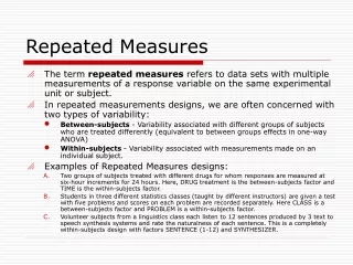
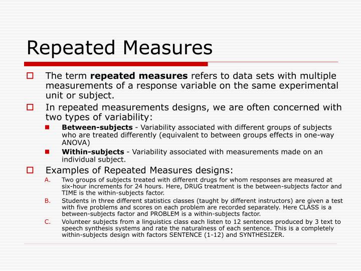
Repeated Measures. The term repeated measures refers to data sets with multiple measurements of a response variable on the same experimental unit or subject. In repeated measurements designs, we are often concerned with two types of variability:

E N D
Repeated Measures • The term repeated measures refers to data sets with multiple measurements of a response variable on the same experimental unit or subject. • In repeated measurements designs, we are often concerned with two types of variability: • Between-subjects - Variability associated with different groups of subjects who are treated differently (equivalent to between groups effects in one-way ANOVA) • Within-subjects - Variability associated with measurements made on an individual subject. • Examples of Repeated Measures designs: • Two groups of subjects treated with different drugs for whom responses are measured at six-hour increments for 24 hours. Here, DRUG treatment is the between-subjects factor and TIME is the within-subjects factor. • Students in three different statistics classes (taught by different instructors) are given a test with five problems and scores on each problem are recorded separately. Here CLASS is a between-subjects factor and PROBLEM is a within-subjects factor. • Volunteer subjects from a linguistics class each listen to 12 sentences produced by 3 text to speech synthesis systems and rate the naturalness of each sentence. This is a completely within-subjects design with factors SENTENCE (1-12) and SYNTHESIZER.
Repeated Measures • When measures are made over time as in example A we want to assess: • how the dependent measure changes over time independent of treatment (i.e. the main effect of time) • how treatments differ independent of time (i.e., the main effect of treatment) • how treatment effects differ at different times (i.e. the treatment by time interaction). • Repeated measures require special treatment because: • Observations made on the same subject are not independent of each other. • Adjacent observations in time are likely to be more correlated than non-adjacent observations
Repeated Measures • Methods of repeated measures ANOVA • Univariate - Uses a single outcome measure. • Multivariate - Uses multiple outcome measures. • Mixed Model Analysis - One or more factors (other than subject) are random effects. • We will discuss only univariate approach
Repeated Measures A layout of simple repeated measures with three treatments on n subjects.
Repeated Measures • Assumptions: • Subjects are independent. • The repeated observations for each subject follows a multivariate normal distribution • The correlation between any pair of within subjects levels are equal. This assumption is known as sphericity.
Repeated Measures • Test for Sphericity: • Mauchley’s test • Violation of sphericity assumption leads to inflated F statistics and hence inflated type I error. • Three common Corrections for violation of sphericity: • Greenhouse-Geisser correction • Huynh-Feldt correction • Lower Bound Correction • All these three methods adjust the degrees of freedom using a correction factor called Epsilon. • Epsilon lies between 1/k-1 to 1, where k is the number of levels in the within subject factor.
Repeated Measures - SPSS Demo • Analyze > General Linear model > Repeated Measures • Within-Subject Factor Name: e.g. time, Number of Levels: number of measures of the factors, e.g. we have two measurements PLUC.pre and PLUC.post. So, number of level is 2 for our example. > Click on Add • Click on Define and select Within-Subjects Variables (time): e.g. PLUC.pre(1) and PLUC.pre(2) • Select Between-Subjects Factor(s): e.g. grp
Repeated Measures - R Demo • Arrangement of the data can be done in MS-Excel. However the following R commands will arrange the data in default.csv for the ANOVA of repeated measures- attach(x) sid1<- c(sid,sid) grp1<-c(grp,grp) plc<- c(PLUC.pre, Pluc.post) time<-c(rep(1,60),rep(2,60)) • The following code is for repeated measures ANOVA summary(aov(plc~factor(grp1)*factor(time) + Error(factor(sid1))))
Repeated Measures R output: Error: factor(sid1) Df Sum Sq Mean Sq F value Pr(>F) factor(grp1) 2 121.640 60.820 16.328 2.476e-06 *** Residuals 57 212.313 3.725 --- Signif. codes: 0 ‘***’ 0.001 ‘**’ 0.01 ‘*’ 0.05 ‘.’ 0.1 ‘ ’ 1 Error: Within Df Sum Sq Mean Sq F value Pr(>F) factor(time) 1 172.952 172.952 33.8676 2.835e-07 *** factor(grp1):factor(time) 2 46.818 23.409 4.5839 0.01426 * Residuals 57 291.083 5.107 --- Signif. codes: 0 ‘***’ 0.001 ‘**’ 0.01 ‘*’ 0.05 ‘.’ 0.1 ‘ ’ 1
Odds Ratio • Statistical analysis of binary responses leads to a conclusion about two population proportions or probabilities. • The odds in favor of an event is the quantity p/1-p, where p is the probability (proportion) of the event. • The odds ratio of an event is the ratio of the odds of the event occurring in one group to the odds of it occurring in another group. • Let p1 be the probability of an event in one group and p2 be the probability of the same event in the other group. Then the odds ratio,
Odds Ratio Estimating odds ratio in 2x2 table The odds of cancer among smokers is a/b and the odds of cancer in non-smokers is c/d and the ratio of two odds is,
Odds Ratio • The odds ratio must be greater than or equal to zero. As the odds of the first group approaches zero, the odds ratio approaches zero. As the odds of the second group approaches zero, the odds ratio approaches positive infinity • An odds ratio of 1 indicates that the condition or event under study is equally likely in both groups. • An odds ratio greater than 1 indicates that the condition or event is more likely in the first group. • An odds ratio less than 1 indicates that the condition or event is less likely in the first group. • Log odds …
Odds Ratio-Demo • MS-Excel: No default function • SPSS: Analyze > Descriptive Statistics > Crosstabs > Select Variables: Row(s): Two groups we want to compare e.g. shades, Column(s): Response variable e.g (pc)> Click on Statistics > Select Risk. • R: Odds ratio are calculated from Logistic regression model.
Logistic Regression • Consider a binary response variable Y with two outcomes (1 and 0). Let p be the proportion of the event with outcome 1. • The logit(p) can be defined as log of odds of the event with outcome 1. Then the logistic regression for the response variable Y on a set of explanatory variables X1, X2, …., Xr can be written as logit(p) = log(p/1-p)= b0 +b1X1+ … +brXr
Logistic Regression • From the model of logistic regression, the odds in favor of Y=1, (p/1-p), can be expressed interms of some r independent variables, p/1-p = exp( b0 + b1X1 + +brXr ) • If there is no influence of the explanatory variables (i.e. X1=0, … Xr =0), the odds in favor of Y=1, (p/1-p), is exp(b0). • If an independent variable (e. g. X1 in the model) is categorical with two categories, then exp(b1) implies the ratio of odds (in favor of Y=1) in two categories of the variable X1. • If an independent variable (e. g. X2 in the model) is numeric, then exp(b2) implies the change in odds (p/1-p) for 1 unit change in X2.
Logistic Regression-Demo • MS-Excel: No default functions • SPSS: Analyze > Regression > Binary Logistic > Select Dependent variable: > Select independent variable (covariate) • R: uses the ‘glm’ function for Logistic regression analysis. Codes are in the R-output slide.
Logistic Regression R output Shades[Shades==2]<-0 > ftc<-glm(pc~Shades, family=binomial(link = "logit")) > summary(ftc) Call: glm(formula = pc ~ Shades, family = binomial(link = "logit")) Deviance Residuals: Min 1Q Median 3Q Max -1.706e+00 -7.290e-01 -1.110e-16 7.290e-01 1.706e+00 Coefficients: Estimate Std. Error z value Pr(>|z|) (Intercept) 1.1896 0.4317 2.756 0.00585 ** Shades -2.3792 0.6105 -3.897 9.73e-05 *** --- Signif. codes: 0 ‘***’ 0.001 ‘**’ 0.01 ‘*’ 0.05 ‘.’ 0.1 ‘ ’ 1 (Dispersion parameter for binomial family taken to be 1) Null deviance: 83.178 on 59 degrees of freedom Residual deviance: 65.193 on 58 degrees of freedom AIC: 69.193 Number of Fisher Scoring iterations: 4 > confint(ftc) Waiting for profiling to be done... 2.5 % 97.5 % (Intercept) 0.3944505 2.114422 Shades -3.6497942 -1.237172 > exp(ftc$coefficients) (Intercept) Shades 3.2857143 0.0926276 > exp(confint(ftc)) Waiting for profiling to be done... 2.5 % 97.5 % (Intercept) 1.48356873 8.2847933 Shades 0.02599648 0.2902037 >