Download
1 / 29
290 likes | 427 Views
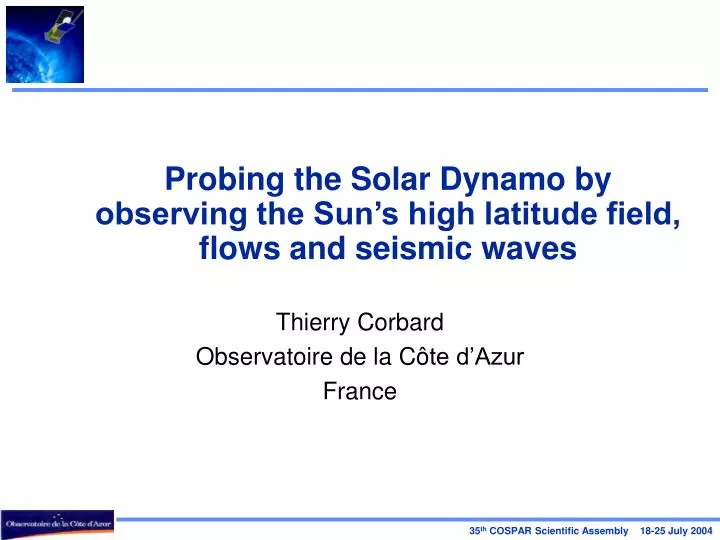
Probing the Solar Dynamo by observing the Sun’s high latitude field, flows and seismic waves. Thierry Corbard Observatoire de la C ô te d’Azur France. Plan. Links between the Solar interior and magnetic cycle Observed Surface Magnetic fields Solar Dynamo models

E N D
Probing the Solar Dynamo by observing the Sun’s high latitude field, flows and seismic waves Thierry Corbard Observatoire de la Côte d’Azur France
Plan • Links between the Solar interior and magnetic cycle • Observed Surface Magnetic fields • Solar Dynamo models • Current helioseismic probe of the dynamo and limitations • Internal angular velocity from Global helioseismology • 3D Subsurface flows from local helioseismology • Perspectives for Solar Orbiter
Observed Surface magnetic Fields Equatoward migration of sunspot-belt Variation of amplitudes, duration etc.. Courtesy: D. Hathaway; NASA/MSFC
Observed Surface magnetic Fields Courtesy: D. Hathaway; NASA/MSFC • Weak diffuse fields outside the sunspot drift poleward • Polar reversal takes place during sunspot maximum • Polar field take the sign of the following spots of the current cycle
Poloidal Field Differential rotation Ω-effect Helical Turbulence (-effect) . Toroidal Field 6 Ingredients for Solar Dynamo Models + Meridional Circulation Parker 1970 + Flux Tube dynamics, buoyancy and stability Parker 75, Fan et al. 93, D’Silva & Choudhouri 93, Caligari et al. 95…
Poloidal Field Differential rotation Ω-effect Helical Turbulence (-effect) Toroidal Field 6 Ingredients for Solar Dynamo Models 2 Main Class of Dynamo models • Flux transport Dynamo(Wang et al. 91, Choudhuri et al. 95, Durney 95…) • Interface Dynamo(Parker 93, Tobias 96, Charbonneau & Mc Gregor 97….) + Meridional Circulation Dikpati & Charbonneau 99, Petrovay & Kerekes 2004 + Flux Tube dynamics, buoyancy and stability
Evolution of Magnetic Fields in a Flux Transport Solar Dynamo Model Courtesy M. Dikpati + Addition of a tachocline -effect is needed to satisfy Hale’s polarity rule (Dikpati & Gilman 2001)
Global Helioseismology Internal Rotation breaks spherical symmetry => Multiplets of 2l+1frequencies Frequency (mHz) : n=3 Unknown n=2 n=1 observed Standard Solar Model n=0 => 2D Inverse Problem Angular degree l
Pole Tachocline Equator “Polar Jet” ? Global Helioseismology Results: Internal Rotation Corbard 98 Schou et al. 2002 Period (days)
Global Helioseismology Results: Torsional Oscillations Adapted from Corbard & Thompson 2001 • Pattern found to persist from the surface down to (0.82R) Howe et al. 2000 • Indications of even deeper penetration at high latitudes Vorontsov et al. 2002 • likely a back reaction from the Dynamo generated magnetic field
Global HelioseismologyLimitations • Sensitive only to the part of the rotation that is symmetric about the equator. • Kernels Independent of longitude (e.g. cannot detect effect of active region on rotation) • Limited access to the polar zone • Impossible to separate the spherically asymmetric effects other than rotation (meridional circulation, magnetic fields, structural asphericity)
Local HelioseismologyAnalysis Principles • Small areas (16ºx16º) are tracked (typically between 8hrs and 28hrs)over the solar disk at a rate depending on the latitude of their center. • These areas are remapped using a Postel or transverse cylindrical projection that tend to preserve the distance along great circles. • => Data cubes (Latitude – Longitude – time)
Local HelioseismologyMain Methods Based on the local observation of global acoustic modes. • Time-distance analysis (Time domain)(Duvall et al. 1993, 1996) • Ring-Diagram analysis (Fourier domain)(Gough & Toomre 1983; Hill 1988) • Acoustic Holography (Phase sensitive) • (Lindsey & Braun, 1990, 1997)
Time-distance helioseismology Principles • First developed by Duvall 1993 • Employs waves travel times observed between different surface location on the Sun. • These travel times are then “inverted” to deduce: • Flow speed and direction, • Sound speed perturbations • [Magnetic field perturbations] Along the ray paths of the observed modes.
Time-distance helioseismology Measuring Travel times • These travel times are obtained by cross-correlating the observed surface oscillations. • Because of the stochastic nature of excitation of the oscillations, the cross-covariance function must be averaged over some areas on the solar surface to achieve a S/N sufficient for measuring travel times. =>Averages are made on rings around the central point Kosovichev & Duvall., 1997
Time-distance helioseismology Interpretation of travel time perturbations Fermat’s Principle and ray approximation theory Phase travel time perturbation Gough 1993 Kosovichev 1996 Ray path in the unperturbated medium Perturbation of the wave number • Bogdan 97: wavepacket are not confined to the raypath • Development of wave-theoretical sensitivity kernels: Jensen et al. (2000), Birch & Kosovitchev (2000), Jensen & Pijpers (2002), Gizon & Birch (2002) • First comparisons (e.g. Couvidat et al. (2004)) show reasonable agreement for depths above 15Mm
Time-distance helioseismology Interpretation of travel time perturbations Dispersion relation: (Kosovichev et al. 1997) Alvén velocity 3D velocity field Acoustic cut off frequency • Temperature perturbations => do not depend on the direction of propagation • Flow perturbations => waves move faster along the flow • Magnetic fields perturbations => waves traveling perpendicular to the field lines are the most sensitive to B (wave speed anisotropy not yet detected) Ryutova & Scherrer 1998
Time-distance helioseismology Inverting Travel Times Maps Annulus ranges: 1º19 - 1º598 +Different annulus ranges sound different depths Zhao 2004 Inversions for sound speed perturbations and 3D flows as a function of depth
Time-distance helioseismology Results: 3D Flows below sunspot 0-3 Mm 6-9 Mm Downward flows Upward flows Zhao, Kosovichev,Duvall 2001 9-12 Mm
Time-distance helioseismology Sub sunspot dynamics and structure Illustration of sound speed variations and subsurface flow patterns of a sunspot The cluster Model of Sunspot Parker 1979 Courtesy SoHO/MDI
Ring Diagram Analysis 3D FFT (, ,t) (kx,ky,) 3D Power spectra Fitting 2 x 1D Inversions Vz may then be computed using the divergence of the horizontal flow and assuming mass conservation. (Komm, Corbard et al. 2004) ky kx
Synoptic Maps of Vorticity – Kinetic Helicity etc.. Komm, Corbard et al. 2004 (ring diagrams) Zhao & Kosovichev 2003 (time-distance)
Time and depth variations ofMeridional Flows Basu & Antia 2002 Gonzalez Hernandez et al. 2004
Controversial detection of a counter cell at “high latitudes” in the Northern hemisphere Haber et al. 2002 Not found by Basu and Antia 2003 And Time-distance analysis Zhao and Kosovichev 2003
Dynamo Models and Polar Reversal N-S asymmetry in meridional flow speed during 1996-2002 and the appearance of a reverse, high-latitude flow cell in the N-hemisphere during 1998-2001 caused the N-pole to reverse ~1 yr before the S- pole Dikpati et al. 2003
Perspectives for The Solar Orbiter • The Visible Light-imager and Magnetograph (VIM) will provide high resolution Magnetograms and Dopplergrams from outside the ecliptic plane (up to 30º). • Immediate benefit: Reduced foreshortening and Increased sensitivity to Magnetic Fields (factor 5) • Possibility of stereoscopic observations with SDO or Earth (120º) • Observations will provide the missing parts of solar dynamo models • Polar rotation rate and torsional oscillation pattern(High latitude Jets?, lower rotation bands migrating poleward ?) • Polar meridional flows (counter cell, returning flow ?) • Maps of high latitude vorticity / kinetic helicity / Small scale Dynamo • Direct observations of polar reversal and flux cancellation processes • Access to the deep layers (tachocline) from stereoscopic observations • Access to the far side of the Sun (continuous probe of spots / far side imaging technique)
Acoustic HolographyFar Side Imaging Lindsey & Braun (1997) A local acoustic depression at the focal point will shift the phase of the ingression-egression correlation.
Concluding Remarks • The field of Local Helioseismology is fairly new • A lot of efforts have been made during the last few years in: • Understanding the forward problem (wave-theoretical sensitivity kernels / Building of artificial data) • Making comparison between the different Methods (group LoHCO) • Understanding errors, methods resolution and correlations • Understanding effects of image misalignment / geometric effects (P-angle / Bo angle) • First Results are very encouraging and positive • First attempt of “archeo-helioseismology” using Mt Wilson data in order to infer the meridional circulation in the past two solar cycles • There is no doubt that a lot more progress will be achieved in developing and understanding these methods before the launch of Solar Orbiter