Download
1 / 34
350 likes | 617 Views
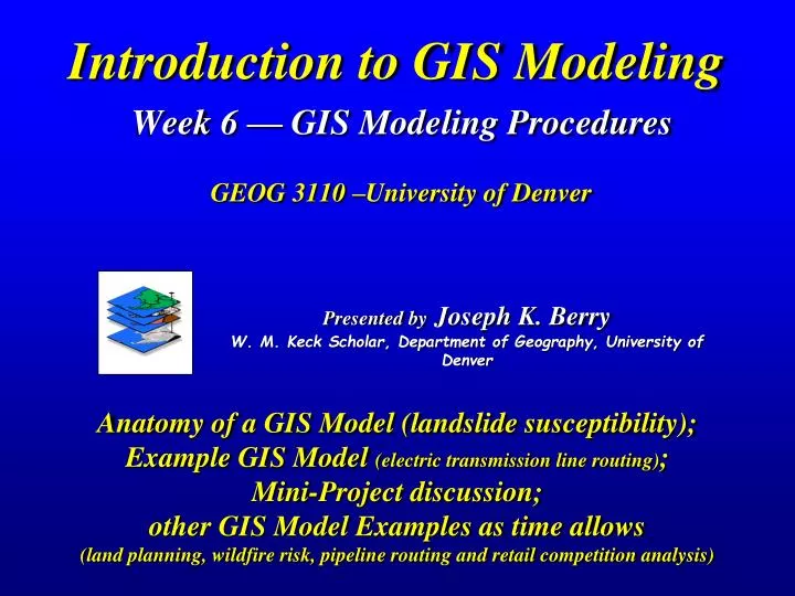
Presented by Joseph K. Berry W. M. Keck Scholar, Department of Geography, University of Denver. Introduction to GIS Modeling Week 6 — GIS Modeling Procedures GEOG 3110 –University of Denver.

E N D
Presented byJoseph K. Berry W. M. Keck Scholar, Department of Geography, University of Denver Introduction to GIS ModelingWeek 6 — GIS Modeling Procedures GEOG 3110 –University of Denver Anatomy of a GIS Model (landslide susceptibility); Example GIS Model (electric transmission line routing); Mini-Project discussion; other GIS Model Examples as time allows (land planning, wildfire risk, pipeline routing and retail competition analysis)
Have a hand calculator or use Window’s Calculator… Start Programs Accessories Calculator Note– Tutor25.rgs, Agdata.rgs, Island.rgs, Bighorn.rgs, GosseEgg.rgs and Smallville.rgs databases are accessed from MapCalc Online Exam 1 (Midterm) This exam is a 2.0 hour, closed book affair taken over the Internet (honor system) — you can take during any 2-hour block after 8:00 am Friday February 12 and must be completed by 5:00 pm Wednesday February 17 (submit via email to jberry@innovativegis.com) You will download the exam from the class website (time/date stamped) and email the completed document to me within 2.0 hours Note that there will be two parts to the exam— answer FIVE questions for Part 1, ONE from Part 2 and ONE from Part 3 Part 250 Points How things work:Choose 1 of the three 25-point questions… Part 1 100 Points Terminology/concepts:Choose any 5 of the seven 20-point questions (i.e., do not answer two) Mini-exercises:Choose 1 of the three 25-point questions (Berry)
Class Logistics and Schedule Midterm Study Questions(hopefully you are participating in a study group) Midterm Exam …you will download and take the 2-hour exam online (honor system) sometime between 8:00 am Friday February 13 and must be completed by 5:00 pm Wednesday February 17 Blue Light Special …20 minutes of Instructor “Help” on midterm study question “toughies “ Exercise #6 (mini-project) — you will form your own teams (1 to 3 members) and tackle one of five projects; we will discuss the project “opportunities” in great detail later in class …assigned tonight Thursday, February 12 and final report due Sunday, February 21 by 5:00pm What should we do about submitting “large” mini-Project Reports …??? No Exercise Week 7— a moment for “dance of celebration” Exercises #7 and #8— to tailor your work to your interests, you can choose to not complete either or both of these standard exercises; in lieu of an exercise, however, you must submit a short paper (4-8 pages) on a GIS modeling topic of your own choosing. Final Exam — to lighten the load at the end of the term, you can choose to forego the final exam; you will receive your average grade for all work to date. Berry
GIS Modeling (Binary Logic; Ranking Model) Binary Choropleth 0, 1 Slope Renumber 0, 1 0, 1 Calculate Renum 0, 1 Renum (Berry)
GIS Modeling (Arithmetic Average; Rating Model refinement) Ratio Choropleth 1 - 9 Renumber 1 - 9 1 - 9 Calculate Renum 1 - 9 Renum (Berry)
GIS Modeling (Simple Buffer Extension) 0, 1 Spread Renumber Calculate (Berry)
GIS Modeling (Effective Buffer Extension) …but what about a refinement that would create a weighted buffer with declining weight factors for increasing distance— 0 = outside buffer 1 = road cell .9 = close to road : = increasing distance .1 = buffer edge cell 0 - 1 0, 1 Spread Renumber Renumber (Berry)
Existing Powerline Goal– identify thebest route for an electric transmission linethat considers various criteria for minimizing adverse impacts. Proposed Substation Houses • Criteria – the transmission line route should… • Avoid areas ofhigh housing density …prefer low housing density • Avoid areas that arefar from roads …prefer close to roads • Avoid areaswithin or near sensitive areas …prefer far from sensitive areas • Avoid areas of highvisual exposure to houses …prefer low visual exposure Roads Sensitive Areas Elevation Houses Transmission Line Routing Model (Hypothetical) (See Beyond Mapping III, Topic 19 for more information) (Berry)
PROPOSED SUBSTATION (END) AVOID AREAS OF HIGH HOUSING DENSITY EXISTING POWERLINE (START) Least preferred (high cost) Most preferred (low cost) MOST PREFERRED ROUTE ACCUMULATED PREFERENCE SURFACE Step 3.The steepest downhill path from the Substation over the Accumulated Preference surface identifies the “most preferred route”— Most Preferred Route avoiding areas of high visual exposure HOUSES HOUSING DENSITY DISCRETE PREFERENCE MAP Step 2.Accumulated Preference from the existing powerline to all other locations is generated based on the Discrete Preference map. Step 1.Housing Density levels (0-83 houses) are translated into values indicating relative preference (1= most preferred to 9=least preferred) for siting a transmission line at every location in the project area. Routing and Optimal Paths (avoid high housing density) Single-criteria Model (Berry)
Withina single map layer Amonga set of map layers Avoid areas of… “Algorithm” “Calibrate” “Weight” High Housing Density …build on this single factor Far from Roads In or Near Sensitive Areas High Visual Exposure Model logic is captured in a flowchart where the boxes represent maps and lines identify processing steps leading to a spatial solution Routing Model Flowchart (Model Logic) Multi-criteria Model (Berry)
Withina single map layer Amonga set of map layers “Algorithm” “Calibrate” “Weight” Step 1 Identify overall Discrete Preference(1 Good to 9 Bad rating) End Start Start Step 2 Generate anAccumulated Preferencesurface from the starting location to everywhere End Step 3 Step 2 Step 1 Step 3 Identify theMost Preferred Routefrom the end location Model logic is captured in a flowchart where the boxes represent maps and lines identify processing steps leading to a spatial solution Routing Model Flowchart (Model Logic) Best Route Route Accumulation Surface (Berry)
Step 1 Discrete Preference Map Calibrate …then Weight HDensity Most Preferred “Pass” RProximity SAreas VExposure …identifies the “relative preference” of locating a route at any location throughout a project area considering all four criteria [avoid areas of High Housing Density, Far from Roads, In/Near Sensitive Areas and High Visual Exposure] Least Preferred “Mountain” of impedance (avoid) Discrete Preference Map Most Preferred (Berry)
Step 2 Accumulated Preference Map …identifies the “total incurred preference” (minimal avoidance) to locate the preferred route from a Starting location to everywhere in the project area Accumulated Preference Map (most preferred) “Pass” (most preferred) “Pass” (digital slide show AccumSurface) Splash Algorithm – like tossing a stick into a pond with waves emanating out and accumulating preference as the wave front moves (Berry)
Step 3 Most Preferred Route …the steepest downhill path from the End over the accumulated preference surface identifies the optimal route that minimizes traversing areas to avoid (most suitable) Optimal Route (most preferred) “Pass” (most preferred) “Pass” (digital video OptimalPath) Note: Straightening and Centering techniques can be applied …see Beyond Mapping III, Topic 19 for more information (Berry)
Step 4 Generating Optimal Path Corridors (digital slide show TotalAccumulation.ppt) …the accumulation surfaces from the Start to the End locations are added together to create a total accumulation surface—the “valley” is flooded to identify the set of nearly optimal routes (most preferred) “Pass” (most preferred) “Pass” Optimal Corridor (Berry)
Combining alternative corridors identifies the decision space reflecting various perspectives Feature Article in GeoWorld, April, 2004 A Consensus Method Finds Preferred Routing See www.geoplace.com/gw/2004/0404/0404pwr.asp Model Results (Georgia Experience ...EPRI, GTC, Photo Science) (Berry)
Routing Model Flowchart Siting Model …maps identifying areas that must be avoided Engineering Natural Environment Built Environment Avoidance Areas Linear Infrastructure Public Lands Building Density Non- Spannable Water bodies State and National Parks Listed NRHP Districts And Buildings Slope Streams/ Wetlands Proximity to Buildings Mines and Quarries (actvie) USFS Wilderness Area City and County Parks Floodplain Spannable Lakes/Ponds Land Cover Proposed Dev.s Buildings Wild/Scenic Rivers Day Care Centers Wildlife Habitat Land Use Airports Wildlife Refuge Cemetery Parcels Military Facilities Listed Archeology Sites School Parcels (K-12) …maps of the criteria for siting are identified, then interpreted by different stakeholder groups for relative importance in routing EPA Superfund Sites Church Parcels Route Engineering 5 times more important Natural 5 times more important Built 5 times more important Simple Average Equally important Weight Calibrate (Berry)
Alternate Corridors …Alternate Corridors for each stakeholder perspective are generated Built Natural Engineering Simple (Average) All (Berry)
Additional Data Collection …extensive site-specific information is gathered within the Alternative Corridor boundaries to aid in refining and selecting final options (Berry)
Generate Alternative Routes (Design Team) Routes are defined within the Alternative Corridors using expert judgment. …Design Team finalizes the Alternate Routes • Objective • Quantitative • Predictable • Consistent • Defensible Exceptions are noted for deviations from optimal paths within the corridor area… Built Natural Engineering Simple …deviations outside the corridor area require variance approval (Berry)
Routing Model Experience (Conclusions) The Methodology is… Objective, Quantitative, Predictable, Consistent, Defensible GIS-based approaches for routing electric transmission lines utilizerelative ratings (calibration)and relative importance (weights)in considering factors affecting potential routes. A quantitative process for establishingobjective and consistent weightsis critical in developing a robust and defendable transmission line siting methodology. Note: there are advance techniques for Calibration and Weighting …link to CalibrateWeight.ppt See www.innovativegis.com/basis/present/GW04_routing/GW_Apr04_routingPowerline.htm Feature Article in GeoWorld, April, 2004 “A Consensus Method Finds Preferred Routing” (Georgia Experience) See www.innovativegis.com/basis, select , online book Beyond Mapping III, Topic 19 “Routing and Optimal Paths” See www.innovativegis.com/basis, select Column Supplements Beyond Mapping, September 03, Delphi (Calibration) See www.innovativegis.com/basis, select Column Supplements Beyond Mapping, September 03, AHP (Weighting) (Berry)
Mini-Project (Exercise #6) Exercise #6 (mini-project) — you will form your own teams (1 to 3 members) and tackle one of eight projects …assigned today and final report due Sunday, February 21 by 5:00pm Project 1 –Hugag Habitat Suitability Revisited Project 2 – Visual Exposure to Timber Harvesting Project 3 – Emergency Response Project 4 – Geo-Business Analysis Project 5 – Landslide Susceptibility Project 6 – Transmission Line Routing Project 7 – Wildfire Risk Analysis Project 8 – Pipeline Spill Migration Project 9–Biomass Accessibility (Berry)
GIS Modeling (Example Project) Example Project – Slippery Mountain Landfill Suitability …criteria for a 0 (not suitable), 1 (minimally suitable) through 9 (extremely suitable) …Your charge is to prepare a prospectus for deriving the Landfill Suitability map that clearly explains how each of criteria are evaluated and then combined into an overall suitability map that respects the legal constraints and reflects the county commissioners’ criteria weightings. In addition, calculate the average landfill suitability rating for each district (Districts map). Finally, generate a map that identifies the average rating within 300 meters (3-cell reach) for each of the housing locations (Housing map). (Berry)
Example Graded Project – Landfill Suitability …posted online at class website, under “Lecture Notes” section, Week 6, Graded Mini-Project Example (Berry)
Hugags like to be near water Hugags are terrified of roads …add four newhabitat criteria Hugags like cover diversity Hugags like to be near forest edges Project 1 – Hugag Habitat Suitability Revisited …implement a weighted average analysis and compare the old and new results (Berry)
…first phase off-road travel by ATV starting at any road location and encountering the following ATV_friction for determining effective proximity …second phase proceeds on foot into the ATV inaccessible areas by using the “Explicitly” option to Spread …final map uniquely identifies ocean (blue) and hiking inaccessible areas (grey), and rescue response time (green to red) as both a 2-D map and a 3-D drape on the elevation surface Project 3 – Emergency Response (Berry)
Competition Analysis Part 1— calculate two travel-time maps, one from Kent’s Emporium and the other from Colossal Mart Part 2— create a relative travel-time advantage map clearly shows which store has the relative advantage Part 3— generate a binary map identifying just the “combat” zone where neither store has a strong advantage Part 4— generate a map that identifies the customers in the combat zone. Density Analysis Part 1— Create a customer density surface that identifies the total number of customers within half a kilometer Part 2— Generate a binary map identifying the “pockets” ofunusually high customer density (mean + 1 Stdev or more customers per 500m reach). Part 3— Generate a map that shows the relative travel-time advantage within the pockets of unusually high customer density. Project 4 – Geo-Business Analysis (Berry)
Project 5 – Landslide Susceptibility …criteria for a 0 (not susceptible), 1 (minimally susceptible) through 9 (extremely susceptible) Overall landslide susceptibility is defined as the weighted average rating of the three criteria A second map that identifies the susceptibility ratings for just the uphill areas around roads to 250 meters (2.5 cells) Another map identifying the average landslide susceptibility (1 to 9) within the uphill buffered area around roads for each of the management districts identified on the Districts map (Berry)
Least Cost Path Accumulated Cost Map Discrete Cost Map Project 6 –Transmission Line Routing • The client, MegaWatt Power, needs to identify three routes— • a route that treats visual exposure from houses and roads equally (simple average Cost), • a route considering visual exposure to houses ten times more important than exposure to roads, and • a route considering visual exposure to roads ten times more important than exposure to houses. (Berry)
Wildfire risk needs be summarized in a couple ways… Calculate the average wildfire risk for each of the districts. Create a map that shows the average wildfire risk within a 300 meter buffer around all housing locations. Project 7 – Wildfire Risk Analysis Wildfire Risk is related to— cover type, terrain and human activity factors …implement the “common sense” idea that locations closer to the fire station at the Ranch community center (Locations base map) ought to have the calculated risk lowered. (Berry)
Project 8 –Pipeline Spill Migration Pipeline Spill is related to— physics, product properties and terrain conditions • Identify the implied steepest downhill spill path for each of the three test locations (Spills map) along the proposed new transmission pipeline and map as a 3D Grid display with all three route individually identified and draped over the Elevation surface. • Identify the minimum path time for a spill anywhere along the entire Proposed route (Pipelines map) and map as a 3D Grid display with the spill density map (10 Equal Ranges contours) draped over the Elevation surface. • Create a map that shows the estimated minimum time for a spill based on the spill time map (created above) to reach all of the impacted areas with the high population HCA (HCA_Hpopulation map). • To illustrate the model’s sensitivity to different products create another minimum time map for the high population HCA that considers crude oil flow instead of water. (Berry)
Roads Forests Project 9 –Biomass Accessibility … “scoping” meeting scheduled for tomorrow, Friday, February 12, 12-4 pm Resource Access. The areas of Pine Beetle remediation are first identified by the level of severity and then characterized by the relative access (effective proximity) considering the intervening conditions and characteristics between the roads and the resource areas identified for remediation. Intervening Considerations Resource Access Intervening Considerations.Terrain steepness, variable-width stream buffers and housing density serve as factors determining a location’s relative suitability for biomass removal, as well as affecting a location’s relative accessibility from the roads. Slope Water Houses (Berry)
GIS Modeling (Mini-Projects) …Good luck!!! There is a “Life-Line” if you get totally stuck. For the price of one grade (drop from 100% possible to 89% possible) I will email you a MapCalc script with the complete solution—you just need to write-up the solution in a “professional, free of grammatical/spelling errors, well-organized, clearly written, succinct manner” that demonstrates your understanding of the processing. General clarification, questions and Life-line requests will be processed via email workdays 8:00-4:00 pm and Saturday/Sunday, 9:00-11:00 am. It behooves you to decide on a project and outline a solution as soon as possible. Note: emergency situations call me at 970-215-0825 (Berry)