Download
1 / 36
360 likes | 497 Views
Criticality in the Olami-Feder-Christensen model: Transients and Epicenters. Carmen P. C. Prado Universidade de São Paulo (prado@if.usp.br). VIII Latin American Workshop on Nonlinear Phenomena LAWNP ’03 - Salvador, Bahia, 2003. Carmen P. C. Prado (USP - SP)

E N D
Criticality in the Olami-Feder-Christensen model: Transients and Epicenters Carmen P. C. Prado Universidade de São Paulo (prado@if.usp.br) VIII Latin American Workshop on Nonlinear Phenomena LAWNP ’03 - Salvador, Bahia, 2003
Carmen P. C. Prado (USP - SP) Josué X. de Carvalho (USP, pos-doc) Tiago P. Peixoto (USP, PhD st) Osame Kinouchi (Rib. Preto, USP) Suani T. R. Pinho (UFBa)
Introduction • SOC & Olami-Feder-Christensen model (OFC) • History • Recent developments • Recent results • Transients • Epicenters (real earthquaques) • Our results
Self-organized criticality Bak, Tang, Wisenfeld, PRL 59,1987/ PRA 38, 1988 Sand pile model • “Punctuated equilibrium” • Extended systems that, under some slow external drive • (instead of evolving in a slow and continuous way) • Remain static (equilibrium) for long periods; • That are “punctuated” by very fast events that leads the systems to another “equilibrium” state; • Statistics of those fast events shows power-laws indicating criticality Drive h( i ) h( i ) + 1 Relaxation if s( i) = h(i+1) - h(i) s( i) s( i) - 2 s(i+1) s(i+1) +11 s(i-1) s(i-1) + 1
Does real sand piles exhibits power-laws? Chicago’s: Jaeger, Liu, Nagel, PRL 62 (89) Jaeger, Nagel, Science 255 (92) Bretz et al, PRL 69 (92) Different sizes & time scales Held et al, PRL 65 (90) Roserdahl, Vekic, Kelly PRE 47 (93) Rice piles (Oslo) Frette et al, Nature 379 (96) A. Malthe-Sørenssen, PRE (96)
Earthquake dynamics is probably the best “experimental ” realization of SOC ideas ... The relationship between SOC concepts and the dynamics of earthquakes was pointed out from the beginning (Bak and Tang, J. Geophys. Res. B (1989); Sornette and Sornette, Europhys. Lett. (1989); Ito and Matsuzaki, J. Geophys. Res. B (1990)) Exhibits universal power - laws Gutemberg-Richter ’s law(energy) P(E) E -B Omori ’s law(aftershocks and foreshocks) n(t) ~ t -A Two distinct time scales& punctuated equilibrium Slow: movement of tectonic plates (years) Fast: earthquakes (seconds)
By the 20 ies scientists already knew that most of the earthquakes occurred in definite and narrow regions, where different tectonic plates meet each other...
k Moving plate i - 1 i i + 1 atrito Fixed plate V Burridge-Knopoff model (1967) Olami et al, PRL68 (92); Christensen et al, PRA 46 (92)
Perturbation: Relaxation: If any of the 4 neighbors exceeds Fth, the relaxation rule is repeated. This process goes on until F < Fth again for all sites of the lattice Modelo Olami-Feder-Christensen (OFC): If some site becomes “active” , that is, if F > Fth, the system relaxes:
The size distribution of avalanches obeys a power-law, reproducing the Gutemberg-Richter law SOC even in the non conservative regime Simulation for lattices of sizes L= 50,100 e 200. Conservative case: = 1/4
While there are almost no doubts about the efficiency of this model to describe real earthquakes, the precise behavior of the model in the non conservative regime has raised a lot of controversy, both from a numerical or a theoretical approach. The nature of its critical behavior is still not clear. The model shows many interesting features, and has been one of the most studied SOC models
First simulations where performed in very small lattices ( L ~ 15 to 50 ) • No clear universality class P(s) ~ s- , = ( ) • No simple FSS, scaling of the cutoff • High sensibility to small changes in the rules (boundaries, randomness) • Theoretical arguments, connections with branching process, absence of criticality in the non conservative random neighbor version of the model hassuggested conservation as an essential ingredient. • Where is the cross-over ? S. Lise, M. Paczuski, PRE 63, 2001, PRE 64, 2001 = 0 model is non-critical = 0.25 model is critical at which value of = c the system changes its behavior ???
First large scale simulation(Grassberger, PRE 49 (1994), Middleton & Tang, PRL 74 (1995) ) • periodic boundary conditions: stationary state is periodic • cross over ( ~ 0.18 ): • small , ordered, period = L2 , dominated by small avalanches ( s=1) • large , still periodic but disordered state • open boundary condition: • also a cross over • small : bulk is ordered in a “periodic” state, s=1, but close to the boundaries there is disorder; most of the epicenters and large avalanches are in the boundaries; • large : the whole lattice is prevented from ordering and large avalanches are also triggered in the interior of the lattice;
Spatial correlation starts from the borders Random initial configuration Josué X. Carvalho
Spatial correlation starts from the borders After 2 x 10⁵ avalanches Josué X. Carvalho
Spatial correlation starts from the borders After 10 x 108 avalanches Josué X. Carvalho
More recent work(B. Drossel, PRL 89, 2002) • The power - law distribution of avalanche sizes results from a complex interplay of several phenomena (part of them already pointed out in earlier papers), including: • boundary driven synchronization and internal desynchronization, • limited float-point precision, • slow dynamics within the steady state • the small size of synchronized regions; • In the ideal situation of infinite floating point precision and L , the avalanche size distribution is dominated by avalanches of size 1 , with the weight of large avalanches decreasing to zero with increasing system size. The model is not critical.
For the lattice model with periodic b.c. • The stationary state is always periodic with all avalanches being of size 1. • The failure to observe this in previous works are due to the small level of desynchronization caused by limited float-point precision. • For the lattice model with open b.c. • The study was concentrates on small values of (~0.10). • In the limits L ,infinite precision, also all avalanches are of size1 (all sites topples with F = Fth).
In 2003, Miller and Boulter found again evidences of the existence of a cross-over G. Miller, C.J. Boulter, PRE 67, 2003 • Cross over x associated with the probability of findingan avalanche with s > 1 , lower bound for c (concentrate on 0.20 < 0.25) • 0.12 x 0.16 • the result was not influenced by increasing the precision • above this cross over , if > x < Fsc> >1 ( 10 -28)
However... • Their results have shown a qualitatively different behavior for the conservative regimeindicating that = 0.25 separates two different types of behavior in the OFC model • although x ~ 0.14, c = 0.25 since x c • the extrapolation procedure is not correct, x = 0.25 (what also leads to c = 0.25) • They observed universal features in the non conserving regime
c Branching rate approach Most of the analytical progress on the RN -OFC used a formalism developed by Lise & Jensen which uses the branching rate (). S Lise, H.J. Jensen, PRL 84, 2001 S. T. R. Pinho, C. P. C. Prado, Bras. J. of Phys. 33 (2003). S. T. R. Pinho, C. P. C. Prado and O. Kinouchi, Physica A 257 (1998). M. Chabanol, V. Hakin, PRE 56 (1997) H.M Bröker, P. Grassberger, PRE 56 (1997) Almost critical O. Kinouchi, C.P.C. Prado, PRE 59 (1999)
Branching rate in OFC and R-OFC One counts the number of supercritical descendents generated when a site topples Remains controversial alternative extrapolation procedures Christensen et al, PRL 87 (2001) de Carvalho and C.P.C. Prado, PRL 87 (2001) J. X. de Carvalho, C. P. C. Prado, Phys. Rev. Lett. 84 , 006, (2000).
Miller and Boulter, PRE 66, (2002) • Layer branching rate i ( , L), • i = 1, ... L/2 indicates the distance of the site from the boundary • L = 1000 (non-conservative), L=700 (conservative) • c = 0.25 • average avalanche sizes: (, L) = 1 - 1/s(, L). • “Control” models (beginning of organization)
The qualitative difference in the behavior of the conservative and non-conservative regimewas also observed in other situations S. Hergarten, H. J. Neugebauer, PRL 88, 2002 showed that the OFC model exhibits sequences of foreshocks and aftershocks, consistent with Omori’ s law, but only in the non-conservative regime!
Transients: J. X. de Carvalho, C.P.C. Prado, Physica A, 321 (2003)
Conservative case red line L = 100 black line L = 400 Stationary state is identified by the mean value of the energy per site After a transient, <Fi,j> fluctuates around a mean value Conservative case • The beginning of stationary state is clearly identified • Transient time scales with L2
Non -conservative case, a = 0.240 red line L = 100 black line L = 200 conservative and non-conservative regimes display qualitatively different behavior during transient • Large fluctuations • Much longer transient, scales Lb, b > 2 (in this case ~ 4) • Initial “bump” scales L2
Non -conservative case, a = 0.240 red line L = 100 black line L = 200 Non -conservative case, a = 0.249 red line L = 100 black line L = 400 Lattice must be large enough to show the “bump” ... Detail of beginning...
Dynamics of the epicenters • S. Abe, N. Suzuki, cond-matt/0210289 • earthquake data of a district of southern California and Japan • area was divided into small cubic cells, each of which is regarded as vertex of a graph if an epicenter occurs in it; • the seismic data was mapped into na evolving random graph; Free-scale behavior of Barabási-Albert type
Free-scale network degree of the node (connectivity) P(k) ~ k - Complex networks describe a wide range of systems in nature and society R. Albert, A-L. Barabási, Rev. Mod. Phys. 74 (2002) Random graph distribution is Poisson
Studied the OFC model in this context 0.240 Clear scaling Shifted upwards for the sake of clarity 0.249 Tiago P. Peixoto, C. P. C. Prado, 2003 L = 200, transients of 10 7, statistics of 10 5
Qualitative diference between conservative and non-conservative regimes 0.249 0..25
L = 300 L = 200 We need a growing network ...
Different cell sizes L = 400, 2 X 2 L = 200, 1 X 1
Distribution of connectivity L = 200, = 0.25 L = 200, = 0.249
Conclusions • Robustness of OFC model to describe real earthquakes • Dynamics of epicenters • Many open questions