Download
1 / 27
270 likes | 393 Views
Developing a Dual-Frequency FM-CW Radar to Study Precipitation. Christopher R. Williams Cooperative Institute for Research in Environmental Sciences (CIRES) University of Colorado at Boulder, and Physical Sciences Division (PSD) NOAA Earth System Research Laboratory (NOAA ESRL),.

E N D
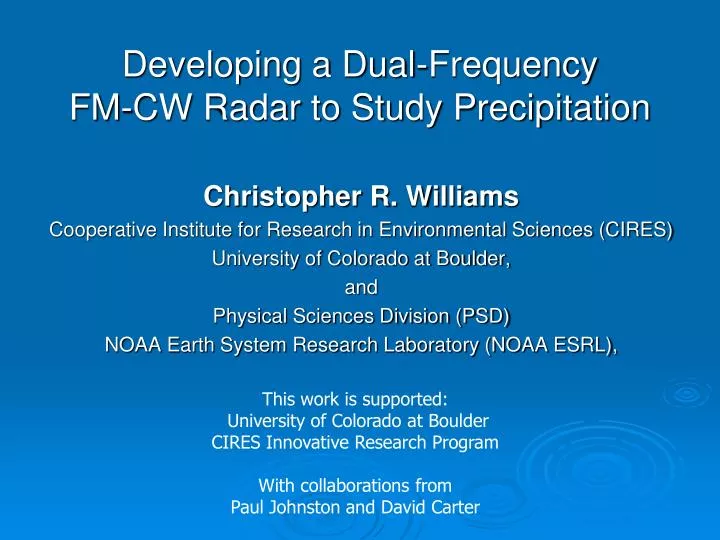
Developing a Dual-Frequency FM-CW Radar to Study Precipitation Christopher R. Williams Cooperative Institute for Research in Environmental Sciences (CIRES) University of Colorado at Boulder, and Physical Sciences Division (PSD) NOAA Earth System Research Laboratory (NOAA ESRL), This work is supported: University of Colorado at Boulder CIRES Innovative Research Program With collaborations from Paul Johnston and David Carter
Motivation • Technically, pulse radars can not observe rain at close ranges as they switch from transmit to receive modes. • Monostatic pulse radars have a “cone of silence” • Proof of concept study to develop an inexpensive radar to observe precipitation between the surface and the first range gate of a pulse radar (~150m). • Bistatic FM-CW radar technology is well suited • Scientifically, raindrops are not uniformly distributed. Raindrops cluster at small spatial and temporal scales due to dynamics and turbulence. • “Cat paws” of raindrops falling on lakes • Mathematically, at what scales should we treat rain as a continuum of raindrops or as discrete objects? • Need to sample to small scales to observe the discrete nature of individual objects
Technology & Methodology • Utilize technologies developed for the mobile phone, the police radar, and the video gaming industries. • One radar operated in the frequency band used for point-to-point Internet service (5.8 GHz). • The other radar operated in the police radar frequency band (10.5 GHz). • A Sony Playstation 3 was used as the numerical workhorse. Installed Linux as Other OS. • The radar hardware for both radar systems cost less than $12k. (no labor costs were included)
Presentation Outline • Hardware Layout • Radar Block Diagram • FMCW Signal Processing • Range Equation • Doppler Processing • Observations
Antennas in my backyard(an understanding wife) C-band Antennas – 5.8 GHz X-band Antennas – 10.4 GHz Antennas are designed for point-to-point Internet service
Hardware Layout Costs for C-band Radar ~$US 6k
Timing Diagram: Frequency Chirp and Data Collection Trigger Sweep Trigger TIPP Tsweep Twait Tdelay Tdwell Tend Frequency Chirp f1 B = f1 - f0 f0 Data Collection Trigger Data is being collected
Timing Equations • Tsweep -Duration the DDS is linearly sweeping from f0 to f1 • Twait -Duration after sweep before next sweep • Allows system to stabilize • TIPP - “Inter-Pulse Period”, time between sweeps • TIPP = Tsweep + Twait • Tipp = 310 us + 10 us = 320 us • Tdwell -Duration the DAS is collecting data • Tdwell = 256 us • Tdelay -Delay until first collected data point data • Want to wait for sweep signal to reach maximum range • Tdelay > 2Rmax / c • Set Rmax = 1.5 km, Tdelay = 10 us
Range Equations For a linear FM signal, a hard target located at range R will generate a delayed version of the transmitted signal t = 2R/c seconds later. Tx Target Rx R
Range Equations For a linear FM signal, a hard target located at range R will generate a delayed version of the transmitted signal t = 2R/c seconds later. Tx Target Rx R Tsweep f1 B = f1 - f0 Tx f0
Range Equations For a linear FM signal, a hard target located at range R will generate a delayed version of the transmitted signal t = 2R/c seconds later. Tx Target Rx R Tsweep f1 Rx B = f1 - f0 Tx f0
Range Equations For a linear FM signal, a hard target located at range R will generate a delayed version of the transmitted signal t = 2R/c seconds later. Tx Target Rx R Tsweep f1 Rx B = f1 - f0 Tx f0
Range Equations The range equation is give by: • B = Sweep frequency bandwidth • Tsweep = Duration of sweep • R = Distance to Target • C = speed of light in free air Frequency resolution determined by Digital Acquisition System (DAS) • Tdwell = time data is collected • n = number of samples • ∆t = time between samples Rearranging the range equation, the range resolution is given by
Range Equations The range resolution: • B = 36.328 MHz • Tsweep = 310 us • n = 128 • ∆t = 2 us Frequency resolution determined by Digital Acquisition System (DAS) n R=(n-1)∆R fIF=(n-1)∆fIF 1 0 DC 2 5 m 3.9 kHz 3 10 m 7.8 kHz 11 50 m 39 kHz 64 315 m 245.7 kHz ∆R = 5 m ∆fIF = 3.9 kHz
Doppler Processing Two FFTs generate Doppler velocity spectra at each range • First FFT is the range-FFT and is applied to the 128 voltages collected during Tdwell • This range-FFT converts the n real valued voltages into complex intermediate frequencies • Range: –fNyquist < fIF < +fNyquist (fNyquist = (2∆t)-1 = 250 kHz) • Spacing: 3.9 kHz • Spectrum is symmetric • Drop negative frequencies which are “Behind” the radar • Rename real and imaginary components “I” and “Q” • Second FFT is the Doppler-FFT and is applied to time series of I’s & Q’s at each range • Similar to pulse radar processing • Time between sweep is same as Inter-pulse Period (Tipp)
Sample Observations • 20 to 300 m height coverage • Need to put the antennas closer together • 5 m resolution • Doppler velocity spectra at each range • System is not calibrated (need to deploy with a disdrometer for absolute calibration) • 65,536 consecutive sweeps • 21 second dwell period
21 Second Dwell during Rain 300 m 5 m resolution Downward Motion Clutter 0 m
21 Second Dwell during Rain 300 m Downward Motion Clutter 0 m
21 & 10.5 Second Dwells Time: 0-21 sec Time: 0-10.5 sec Time: 10.5-21 sec
5 second Dwells Time: 0-5 sec Time: 5-10 sec Time: 10-15 sec Time: 15-20 sec
21 Second Dwell processed into 1 second intervals 21 Seconds
C- and X-band Observations During Snow A snow event passed over my house on 13 November 2009 and was observed by both the C-band and X-band radars. The X-band transmitted power was limited due to a bad amplifier which reduced its altitude coverage. C-Band Radar X-Band Radar
Key Design Elements There are 3 key design elements • The Data Acquisition System (DAS) commands all time signals and collects all data so that the sample voltage phases are coherent from sweep-to-sweep • The FM bandwidth and DAS sampling frequency control the range resolution allowing the DAS sampling frequency to be only 500 kHz • Doppler velocity power spectra are generated at each range using 2 FFTS: one range-FFT applied to each FM sweep followed by a Doppler-FFT that detects the phase changes over several FM sweeps
Concluding Remarks • Key Result: Proof of Concept was a Success • Separate the two radars so that they have their own data acquisition system • Remove the Sony Playstation 3 (SP3) as the numerical workhorse • Sony prohibits the installation of Linux on the SP3 (since 2010) • GPU’s can be used if intense signal processing is needed • Plan to use FPGA for range-FFT • Need to calibrate system with a disdrometer • Acquired funds to develop a 915 MHz wind profiler to measure winds in the lowest 300 meters