Download
1 / 18
180 likes | 320 Views
What Types Of Data Are Collected?. Research Is A Partnership Of Questions And Data. “Categorical” Data. “Continuous” Data. S010Y: Answering Questions with Quantitative Data Class 2: II.1 Displaying and Summarizing Categorical Data. What Kinds Of Question Can Be Asked Of Those Data?.

E N D
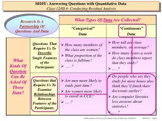
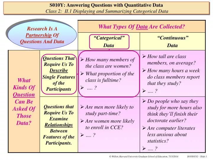
What Types Of Data Are Collected? Research Is A Partnership Of Questions And Data “Categorical” Data “Continuous” Data S010Y: Answering Questions with Quantitative DataClass 2: II.1 Displaying and Summarizing Categorical Data What Kinds Of Question Can Be Asked Of Those Data? Questions That Require Us To Describe Single Features of the Participants • How many members of the class are women? • What proportion of the class is fulltime? • …. ? • How tall are class members, on average? • How many hours a week do class members report that they study? • …. ? Questions that Require Us To Examine Relationships Between Features of the Participants. • Are men more likely to study part-time? • Are women more likely to enroll in CCE? • …. ? • Do people who say they study for more hours also think they’ll finish their doctorate earlier? • Are computer literates less anxious about statistics? • …. ?
Baldus, Pulaski & Woodworth. A Comparative Review of Death Sentences: An Empirical Study of the Georgia Experience, J. Crim. Law, (1983). McCleskey appeals up through the Supreme Court, arguing his death sentence is due to racial bias in sentencing … his appeal is rejected (1987) Julius Chambers, NAACP Legal Counsel testifies at US Senate Committee on the Judiciary (1989) Senator Edward Kennedy sponsors the Racial Justice Act to enforce the “Constitution’s promise of equality under the law” (1989) McCleskey executed in Georgia (1991) On his deathbed, Justice Powell changes his mind!! Here’s the storybehind the data used in our first example… Warren McCleskey is sentenced to death for murdering a policeman during an armed robbery in Georgia (1978) S010Y: Answering Questions with Quantitative DataClass 2: II.1 Displaying and Summarizing Categorical Data
A Codebook describing the contents of the death penalty dataset is in the DEATHPEN_info file. • Racial Bias In Death Penalty Sentencing • We’ll use part of the quantitative data accumulated by Baldus et al. (1983) – in order to: • Introduce simple quantitative methods for describing and summarizing quantitative data that are categorical. • Learn how to write a PC-SAS program to conduct those analyses. S010Y: Answering Questions with Quantitative DataClass 2: II.1 Displaying and Summarizing Categorical Data The death penalty data themselves are contained in the DEATHPEN.txtfile. The Data-Analytic Handout containing the PC-SAS program and output from the death penalty analyses is contained in the Class02/Data Analytic Handout1file
Column #3contains data that tells us the Race of the Victim: • 1 = Black • 2 = White • Column #1contains data that indicates whether the defendant was sentenced to death: • 0 = no • 1 = yes • Column #2contains data that tells us the Race of the Defendant: • 1 = Black • 2 = White • Each row of the dataset contains information on one person: • Each one is a convicted murderer in Georgia. • There are a total of 2475 cases, in this sample. Let’s examine the dataset first … typically, all quantitative data files look like big elongated rectangles … Each column of the dataset contains a different piece of information S010Y: Answering Questions with Quantitative DataClass 2: II.1 Displaying and Summarizing Categorical Data 0 1 1 0 1 1 0 1 1 0 1 1 . . (2475 cases total) . . 1 2 2 1 2 2 • Vocabulary Items: • Each column as a variable. • Entries in the columns are the values of each variable. • These three variables are all categorical. • Subsequently, we will refer to these variables by the following variable names: • DEATH (Column #1) • RDEFEND (Column #2) • RVICTIM (Column #3) In the data file, columns are separated by a space so that the computer can tell them apart!
Questions That Ask You to Describe Single Variables: • How many convicted defendants were sentenced to death? How many were not? • What percentage of convicted murderers were Black? What percentage were White? • What proportion of murder victims were Black? What proportion were White? • Questions That Inquire About Relationships Between Two or More Variables: • Is it more probable that a convicted murderer will be sentenced to death if he is Black, or if he is White? • Is it more probable that a convicted murderer will be sentenced to death if he kills someone Black, or kills someone White? • If a murderer is Black and kills someone White, is it more probable that he will be sentenced to death than if he kills someone Black? How about White murderers? Even though these categorical data are very simple, they invite a variety of interesting research questions about the allocation of the death penalty in Georgia … RVICTIM RDEFEND S010Y: Answering Questions with Quantitative DataClass 2: II.1 Displaying and Summarizing Categorical Data DEATH 0 1 1 0 1 1 0 1 1 0 1 1 . . (2475 cases total) . . 1 2 2 1 2 2
The simplest thing you can do is just list out the data… S010Y: Answering Questions with Quantitative Data Class 2/Handout 1: Displaying and Summarizing Categorical data Death penalty and race bias in Georgia Data in DEATHPEN.txt List values of variables for first 30 cases, w/out value labels Race of Race of Sentenced Obs defendant victim to death? 1 1 1 0 2 1 1 0 3 1 1 0 4 1 1 0 5 1 1 0 6 1 1 0 7 1 1 0 8 1 1 0 9 1 1 0 10 1 1 0 11 1 1 0 12 1 1 0 13 1 1 0 14 1 1 0 15 1 1 0 16 1 1 0 17 1 1 0 18 1 1 0 19 1 1 0 20 1 1 0 21 1 1 0 22 1 1 0 23 1 1 0 24 1 1 0 25 1 1 0 26 1 1 0 27 1 1 0 28 1 1 0 29 1 1 0 30 1 1 0 S010Y: Answering Questions with Quantitative DataClass 2: II.1 Displaying and Summarizing Categorical Data
Or you can “format” the data and list it out … S010Y: Answering Questions with Quantitative Data Class 2/Handout 1: Displaying and Summarizing Categorical data Death penalty and race bias in Georgia Data in DEATHPEN.txt List values of variables for first 30 cases, w/ value labels Race of Race of Sentenced Obs defendant victim to death? 1 Black Black No 2 Black Black No 3 Black Black No 4 Black Black No 5 Black Black No 6 Black Black No 7 Black Black No 8 Black Black No 9 Black Black No 10 Black Black No 11 Black Black No 12 Black Black No 13 Black Black No 14 Black Black No 15 Black Black No 16 Black Black No 17 Black Black No 18 Black Black No 19 Black Black No 20 Black Black No 21 Black Black No 22 Black Black No 23 Black Black No 24 Black Black No 25 Black Black No 26 Black Black No 27 Black Black No 28 Black Black No 29 Black Black No 30 Black Black No S010Y: Answering Questions with Quantitative DataClass 2: II.1 Displaying and Summarizing Categorical Data
S010Y: Answering Questions with Quantitative Data Class 2/Handout 1: Displaying and Summarizing Categorical data Death penalty and race bias in Georgia Data in DEATHPEN.txt Univariate Displays and Summaries of RDEFEND, RVICTIM and DEATH Frequency of DEATH ___ /_ /‚ ‚**‚ ‚ ‚**‚ ‚ ‚**‚ ‚ ‚**‚ ‚ ‚**‚ ‚ ƒ‚**‚ ‚ƒƒƒƒƒƒƒƒƒƒƒƒƒƒƒƒƒƒƒƒƒ / ‚**‚ ‚ / / / ‚**‚ ‚ / ___ / / ‚**‚ ‚ / /_ /‚ / / ‚**‚/ / ‚**‚/ / / / / / 2347 / 128 / /ƒƒƒƒƒƒƒƒƒƒƒƒƒ/ƒƒƒƒƒƒƒƒƒƒƒƒƒ/ No Yes Sentenced to death? The data start to look more interesting when you display them in imaginative ways … • Here’s a Block Chartof the values of the variable that describes Death Penalty Sentencing (DEATH). • The height of each block displays the sample frequencies of the murderer’s sentences, by their type. S010Y: Answering Questions with Quantitative DataClass 2: II.1 Displaying and Summarizing Categorical Data From our Block Chart of the values of variable DEATH, we conclude that: “The sample proportion of convicted murderers who are actually sentenced to death is very small, around .05” • Proportions can also provide useful summary statistics for categorical data: • What proportion of defendants are sentenced to death?
S010Y: Answering Questions with Quantitative Data Class 2/Handout 1: Displaying and Summarizing Categorical data Death penalty and race bias in Georgia Data in DEATHPEN.txt Univariate Displays and Summaries of RDEFEND, RVICTIM and DEATH Race of victim Cum. Cum. Freq Freq Percent Percent ‚ Black ‚****************************** 1502 1502 60.69 60.69 ‚ White ‚******************* 973 2475 39.31 100.00 ‚ Šƒƒƒƒƒƒƒˆƒƒƒƒƒƒƒˆƒƒƒƒƒƒƒˆƒƒƒƒƒƒ 400 800 1200 Frequency • Here’s a Horizontal Histogramof the values of the variable that describes the Race of the Victim (RVICTIM). • The length of each bar displays the frequencywith which victims appear in the sample, on the horizontal axis, by their race. S010Y: Answering Questions with Quantitative DataClass 2: II.1 Displaying and Summarizing Categorical Data • Percentages are useful for summarizing the values of categorical variables across the sample: • What percentage of victims are Black? • What percentage of victims are White? Inspecting the horizontal histogram of values of the variable RVICTIM, and its accompanying percentages, we conclude that … “In the sample of convicted murderers in Georgia, the percentage of murderers with victims who were Black (60.7%) was almost double the percentage of murderers with victims who were White (39.3%).”
S010Y: Answering Questions with Quantitative Data Class 2/Handout 1: Displaying and Summarizing Categorical data Death penalty and race bias in Georgia Data in DEATHPEN.txt Univariate Displays and Summaries of RDEFEND, RVICTIM and DEATH Frequency ‚ ***** 1600 ˆ ***** ‚ ***** ‚ ***** ‚ ***** 1400 ˆ ***** ‚ ***** ‚ ***** ‚ ***** 1200 ˆ ***** ‚ ***** ‚ ***** ‚ ***** 1000 ˆ ***** ‚ ***** ‚ ***** ‚ ***** 800 ˆ ***** ***** ‚ ***** ***** ‚ ***** ***** ‚ ***** ***** 600 ˆ ***** ***** ‚ ***** ***** ‚ ***** ***** ‚ ***** ***** 400 ˆ ***** ***** ‚ ***** ***** ‚ ***** ***** ‚ ***** ***** 200 ˆ ***** ***** ‚ ***** ***** ‚ ***** ***** ‚ ***** ***** Šƒƒƒƒƒƒƒƒƒƒƒƒƒƒƒƒƒƒƒƒƒƒƒƒƒƒƒƒƒƒƒ Black White Race of defendant • Here’s a Vertical Histogramof the values of the variable that describes the Race of the Defendant(RDEFEND). • The height of each bar displays the sample frequencyof defendants, on the vertical axis, by their race. S010Y: Answering Questions with Quantitative DataClass 2: II.1 Displaying and Summarizing Categorical Data Inspecting this vertical histogram of the values of the variableRDEFEND, we conclude that … “In the sample of convicted murderers in Georgia, there are about twice as many Black defendants as there are White defendants.”
Program-wide options Specify titling for the output Data-input paragraph Format key variables Data-analysis “procedure” paragraphs Don’t forget to run the program How did I get all these charts and statistics? … I wrote and executed a PC-SAS program … OPTIONS NodatePageno=1; TITLE1 'S010Y: Answering Questions with Quantitative Data'; TITLE2 'Class 2/Handout 1a: Displaying and Summarizing Categorical data'; TITLE3 'Death penalty and race bias in Georgia'; TITLE4 'Data in DEATHPEN.txt'; *-------------------------------------------------------------------------* Input data, name and label variables in dataset *-------------------------------------------------------------------------*; DATA DEATHPEN; INFILE 'C:\DATA\S010Y\DEATHPEN.txt'; INPUT DEATH RDEFEND RVICTIM; LABEL DEATH = 'Sentenced to death?' RDEFEND = 'Race of defendant' RVICTIM = 'Race of victim'; *-------------------------------------------------------------------------* Format labels for values of categorical variables *-------------------------------------------------------------------------*; PROC FORMAT; VALUE DLABELS 0 = 'No' 1 = 'Yes'; VALUE RLABELS 1 = 'Black‘ 2 = 'White'; *-------------------------------------------------------------------------* List data for subsample of 30 cases, with and without value labels *-------------------------------------------------------------------------*; PROC PRINT LABEL DATA=DEATHPEN(obs=30); TITLE5 'List values of variables for first 30 cases, w/out value labels'; VAR RDEFEND RVICTIM DEATH; PROC PRINT LABEL DATA=DEATHPEN(obs=30); TITLE5 'List values of variables for first 30 cases'; FORMAT DEATH DLABELS. RDEFEND RVICTIM RLABELS.; VAR RDEFEND RVICTIM DEATH; *-------------------------------------------------------------------------* Display summary charts and statistics for entire sample *-------------------------------------------------------------------------*; PROC CHART DATA=DEATHPEN; TITLE5 'Univariate Displays and Summaries'; FORMAT DEATH DLABELS. RDEFEND RVICTIM RLABELS.; VBAR RDEFEND / DISCRETE; HBAR RVICTIM / DISCRETE; BLOCK DEATH / DISCRETE; RUN; S010Y: Answering Questions with Quantitative DataClass 2: II.1 Displaying and Summarizing Categorical Data
Exercising program-wide options: • Include an options line in every program. • The option Nodateeliminates the printing of the date at the head of each page of output. • The option Pageno = # provides the starting page number for the output. • There are dozens of other options, please see the on-line documentation. • Ending each line of the program: • Each “conceptual line of code” ends in a semicolon. • Titling your output: • The output contains titles at the head of each page of output. • You can specify as many titles as you like … TITLE1, TITLE2, TITLE3, etc. • Choose titles in a consistent way, to make your output sensible later. • Content of each title is contained within single quotes, ‘… … …’. • Each title command line ends in a semicolon. First, let’s examine the program-wide options and titling statements: S010Y: Answering Questions with Quantitative DataClass 2: II.1 Displaying and Summarizing Categorical Data OPTIONS Nodate Pageno=1; TITLE1 'S010Y: Answering Questions with Quantitative Data'; TITLE2 'Class 2/Handout 1a: Displaying and Summarizing Categorical data'; TITLE3 'Death penalty and race bias in Georgia'; TITLE4 'Data in DEATHPEN.txt';
Commenting your program: • Add comments to make program more legible. • Start each comment with asterisk (*), end with a semicolon. • You can extend a comment over several physical lines. • Nicknaming the DATA set: • Begin line with the command DATA. • Follow with nickname of your own choosing, here DEATHPEN. • SAS uses the nickname to refer to the dataset subsequently while executing. • I usually choose a nickname that is same as the dataset filename. • Identifying the external datafile: • INFILE command identifies location of the data file on your computer. • Must be a fully qualified data file name, contained in single quotes. • See handout on data-entry on website. • Providing variable labels: • LABEL command provides a label associated with each variable’s name. • Each label can be up to 40 characters. • The actual label is contained in single quotes. • Notice that the entire LABEL “line” can cover more than one physical line. • Providing variable names: • INPUT command names the columns of data (variables) in the order in which they appear in external data file. • Each variable must be given a unique name of up to eight alphanumeric characters, beginning with a letter.. Next examine the data-input paragraph … S010Y: Answering Questions with Quantitative DataClass 2: II.1 Displaying and Summarizing Categorical Data *-----------------------------------------------* Input data, name and label variables in dataset *-----------------------------------------------*; DATA DEATHPEN; INFILE 'C:\DATA\S010Y\DEATHPEN.txt'; INPUT DEATH RDEFEND RVICTIM; LABEL DEATH = 'Sentenced to death?' RDEFEND = 'Race of defendant' RVICTIM = 'Race of victim';
PROC FORMAT: • Procedure to label the values of a variable. • Very flexible, instead of actually labeling the values of a named variable, you create a list of valueformats. • Any format list can be associated with any variable later in the program. • VALUEs: • Each format list begins with the command, VALUE and has its own name, DLABELS, RLABELS, etc. • Each format list contains: • The value to be labeled (e.g., 0), • An equals sign, • The label in quotes (e.g., ‘No’) • Repeat until you have created a label for every value in the set. • Each label can be up to 16 characters. Next, examine the formatting procedure that labels the values of the variables … DATA DEATHPEN; INFILE 'C:\DATA\S010Y\DEATHPEN.txt'; INPUT DEATH RDEFEND RVICTIM; LABEL DEATH = 'Sentenced to death?' RDEFEND = 'Race of defendant' RVICTIM = 'Race of victim'; *------------------------------------------------* Format labels for values of categorical variables *------------------------------------------------*; PROC FORMAT; VALUE DLABELS 0 = 'No‘ 1 = 'Yes'; VALUE RLABELS 1 = 'Black‘ 2 = 'White'; S010Y: Answering Questions with Quantitative DataClass 2: II.1 Displaying and Summarizing Categorical Data
Extra titling: • You can add extra titles as the program continues. • Identifying the variables to be printed: • The VAR command specifies the variables that you want printed (here RDEFEND, RVICTIM & DEATH). • They will be printed out in the order in which they are listed in the VAR line. • Printing out the data: • PROC PRINT is a SAS procedure for printing out datasets (or parts of datasets). • The LABEL option indicates that you want each printed column to be headed by the variable’s label. • The DATA = option identifies the dataset to be printed, by its nickname. • The (obs = #) qualification to the DATA= option limits the number of cases printed. If you omit it, all cases are printed (here, that’s 2475 cases!). Next, examine the first set of data-analyses, which print out the data … *-------------------------------------------------------------------------* List data for subsample of 30 cases, with and without value labels *-------------------------------------------------------------------------*; PROC PRINT LABEL DATA=DEATHPEN(obs=30); TITLE5 'List values of variables for first 30 cases, w/out value labels'; VAR RDEFEND RVICTIM DEATH; PROC PRINT LABEL DATA=DEATHPEN(obs=30); TITLE5 'List values of variables for first 30 cases’; FORMAT DEATH DLABELS. RDEFEND RVICTIM RLABELS.; VAR RDEFEND RVICTIM DEATH; S010Y: Answering Questions with Quantitative DataClass 2: II.1 Displaying and Summarizing Categorical Data
Printing out the data, formatted: • The second time we print out the data, we format it using the format lists created earlier with the PROC FORMAT statement. • Begin the line with the FORMAT command. • Then, list each variable you would like formatted followed by the format you want to use (here DEATH is formatted using DLABELS). • Notice that you need a period immediately after (no space) each format used (it’s a mystery?). Next, examine the first set of data-analyses, to print out the data in the dataset … *-------------------------------------------------------------------------* List data for subsample of 30 cases, with and without value labels *-------------------------------------------------------------------------*; PROC PRINT LABEL DATA=DEATHPEN(obs=30); TITLE5 'List values of variables for first 30 cases, w/out value labels'; VAR RDEFEND RVICTIM DEATH; PROC PRINT LABEL DATA=DEATHPEN(obs=30); TITLE5 'List values of variables for first 30 cases'; FORMAT DEATH DLABELS. RDEFEND RVICTIM RLABELS.; VAR RDEFEND RVICTIM DEATH; S010Y: Answering Questions with Quantitative DataClass 2: II.1 Displaying and Summarizing Categorical Data
Create charts summarizing the data: • PROC CHART is a SAS procedure that will create a variety of summary charts for categorical data. • Need to specify the dataset to be used in a DATA= option. • Then, list each variable you would like formatted followed by the format you want to use (here DEATH is formatted using DLABELS). • Notice that you need a period immediately after (no space) each format used (why?). Here’s the usual titling and formatting • Vertical Bar Chart (Histogram): • The VBAR option produces a vertical histogram of variable RDEFEND. • Need to include the DISCRETE option to let SAS know that RDEFEND is a categorical variable Next, examine the second set of data-analyses, to produce summary charts of the data … S010Y: Answering Questions with Quantitative DataClass 2: II.1 Displaying and Summarizing Categorical Data *-------------------------------------------------------------------------* Display summary charts and statistics for entire sample *-------------------------------------------------------------------------*; PROC CHART DATA=DEATHPEN; TITLE5 'Univariate Displays and Summaries; FORMAT DEATH DLABELS. RDEFEND RVICTIM RLABELS.; VBAR RDEFEND / DISCRETE; HBAR RVICTIM / DISCRETE; BLOCK DEATH / DISCRETE;
Horizontal Bar Chart (Histogram): • The HBAR option produces a horizontal histogram of variable RVICTIM. • Need to include the DISCRETE option to let SAS know that RVICTIM is a categorical variable • Block Chart: • The BLOCK option produces a block chart of variable DEATH. • Need to include the DISCRETE option to let SAS know that DEATH is a categorical variable Producing horizontal bar and block charts … S010Y: Answering Questions with Quantitative DataClass 2: II.1 Displaying and Summarizing Categorical Data *-------------------------------------------------------------------------* Display summary charts and statistics for entire sample *-------------------------------------------------------------------------*; PROC CHART DATA=DEATHPEN; TITLE5 'Univariate Displays and Summaries'; FORMAT DEATH DLABELS. RDEFEND RVICTIM RLABELS.; VBAR RDEFEND / DISCRETE; HBAR RVICTIM / DISCRETE; BLOCK DEATH / DISCRETE;