Download
1 / 26
260 likes | 423 Views
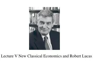
Lecture V New Classical Economics and Robert Lucas. Attack on Keynesianism (again). Like the monetarists before them, the new classical economists also set their sights on Keynesian theory, which they view as simplistic and damaging to the economy

E N D
Attack on Keynesianism (again) • Like the monetarists before them, the new classical economists also set their sights on Keynesian theory, which they view as simplistic and damaging to the economy • Quite opposite to the monetarists, however, new classical theory restates the classical dichotomy of the neutrality of money (although unanticipated monetary shocks can have real affects) • The rational expectations theory used by new classical economists replaces adaptive expectations, which will lead to consistently biased estimates of economic variables • The economist most closely associated with new classical theory is Robert Lucas, Jr.
Rational expectations • The basis of the new classical approach is the idea that expectations are formed “rationally” • It has been argued that it was a stroke of genius to declare your theory to be “rational”; after all, by implication any alternative theory must be irrational, and no one wants to go there • By rational expectations we mean that on average economic agents correctly perceive economic variables • Thus, for example, on average workers will accurately guess the inflation rate next period and will act in such a way as to protect themselves from any adverse effects this will cause them • It does not mean, as some have claimed, that predictions are always correct or that everyone’s predictions are accurate
Origin of rational expectations • The seminal paper on rational expectations was John Muth’s 1961 Econometrica article Rational Expectations and the Theory of Price Movements • Lucas used the theory of rational expectations to account for the apparent non-neutrality of money • According to his formulations, in a world of money surprises, real effects can occur but only to the extent that these surprises are unanticipated • He then showed operationally how to decompose monetary shocks into two components: an anticipated, or forecastable component, and an unanticipated component • Only the unanticipated component should have real effects
Other adopters of RET • Thomas Sargent and Neil Wallace used RET to develop the Policy Ineffectiveness Proposition, or PIP, which shows that if agents use all information efficiently and expectations are realized, on average, then discretionary policies will quickly lose their ability to affect real economic variables • Even New Keynesians, such as Stanley Fisher, adopted RET in their economic models
The simple RET model • Let us suppose we wish to forecast the rate of inflation p • We start with the assumption that economic agents use any and all information available to forecast next period’s inflation rate, which, it is assumed, has one unique value • If the forecast is unbiased then p = p* + u and E(p) = p*, where p is the forecast value of inflation, p* is the actual value, and u is random error with E(u) = 0 and is independent of p* • An alternative, more realistic model, assumes that each agent uses information up to the point that the marginal cost of the additional information equals the marginal benefit; this is the weak form of the so-called efficient market hypothesis • The assumption that all information is used is the strong form of EMH
Criticism 1 • Model assumes a unique p*; in the real world multiple p* may be possible and which p* occurs is based on agents’ actions • For example, the Fed announces a 5% target inflation rate, which is now 10% • if people do not believe the Fed and expect 10% inflation, wage rise 10% and inflation is 10% • If the Fed, however, cuts money growth to coincide with their target 5%, a recession follows • On the other hand, if the Fed credible, then the expected p* is 5% and wages and prices rise by 5% and there is nor recession • Thus, economic agents’ actions may determine p*
Criticism 2 • It is well known that assumptions about individual behavior do not carry over to aggregate behavior • Thus, even if all households and firms are rational (and don’t believe the Fed will hit its 5% inflation target in the previous example) they may still not act on those beliefs • So households, in order to be sure they don’t lose their jobs IF the Fed meets the target, they may accept a 5% wage increase • And firms may only raise their prices 5%, just in case the target is met so as not to have their prices undercut by other firms
Credibility • As noted in both of the previous examples, people’s perceptions of whether or not the central bank will be abel to “stick to its guns” and hold the line on inflation, is critical in whether or not people act in a way to achieve the desired equilibrium • Much of the literature today concerns itself with the issue of central bank credibility, which is based on central bank independence, or CBI
Mark I Example • In Lucas’ early work, his models were based on unanticipated nominal shocks as being the primary source of macroeconomic instability; the was referred to as monetary equilibrium business cycle theory, or MEBCT • As noted earlier, only the unanticipated component of nominal changes could impact real variables, as agents will shield themselves against the anticipated component
A Lucasian Model • Yy = YNt + YCt, where YN is the secular component of GDP and YC is the cyclical component • YNt = λ + φt is the underlying trend growth path of the economy • The cyclical component depends of the surprise and last periods deviation from its natural rate • YCt = α[Pt – E(Pt|Ωt-1)] + β(Yt – YNt-1) • Ω represents all variables used to predict P, and β > 0 determines the speed with which output returns to its natural rate after a shock.
To explain why output and employment remain persistently above or below their trend values for a succession of time periods, further assumptions are made about the propagation mechanism. • These make reference to lagged output, investment accelerator effects, information lags and the durability of capital goods, contracts that inhibit immediate adjustment and adjustment costs. In the filed of employment, firms may face costs both in hiring and firing labor, interviewing and training new employees, making redundancy payments, etc. [Later we shall see that New Keynesians refer to many of the same factors in their models] • As a result firms may adjust employment and output gradually over a period of time after an unanticipated shock
Combining we get Yt = λ + φt + α[Pt – E(Pt|Ωt-1)] + β(Yt – YNt-1) + εt, where εt is a random error process • To account for how accustomed agents in a country are to demand shocks Lucas adds a factor θ to account for speed of adjustment as follows: • Yt = λ + φt + θα[Pt – E(Pt|Ωt-1)] + β(Yt – YNt-1) + εt, the larger the θ, in a country that has not had many inflation shocks, the greater the output impact of price shocks. For example, in countries with lots and variable rates of inflation COLAs will be built into their contracts, so misperceptions are far less of an issue than in a country that has not experienced much inflation. • In his model, the greater the variability in prices, that is, the less that as attributed relative price variability, the smaller the cyclical response of output to a monetary variation.
If the authorities announce and are believed • Suppose the authorities announce they will increase the money supply • If agents believe the announcement, then workers will insist on higherwages as AS moves from AS to AS' and AD will shift outward from AD toAD • Aggregate output remains the same at YN and prices risedirectly from to P2.
Unannounced or not believed • Now if agents do not believe the authorities, or if the central bank does notannounce the monetary increase, then agents believe the increased wagesand product demand to be relative • At first producers increase output, perhaps by paying more for overtime hours, and consumers buy more • Thisshifts AD outward to AD' and price rises to P1 • Then as workers and producers see the higher prices, they insist on higher wages which can be paid at the higher prices
Phillips curve • In the first case, even in the short run, the increased money supply had no effect on output or prices • In the second case, the results are the same as under adaptive expectations; first an increase in output without wage increases, then an increase in wage rate and a decline in output to its original level • This is the story of the short-run versus long-run Phillips curve
Mathematics of the reduced-form Phelps-Friedman PC p = inflation rate U = unemployment rate UN = natural rate of unemployment S = exogenous supply shock D = exogenous demand shock m = money growth pt = pet – φ(Ut – UNt) + φθSt So Ut = UNt -1/ φ(pt - pet) +φθSt pt = mt + θDt is the structural relationship between money and prices, ie. MV=PY
pet = met is rational expectation of the inflation rate • mt = λ0 + λ1(Ut-1 – UN(t-1)) + θmt is the monetary authority money growth response function; if unemployment is above the natural rate, they will increase money growth, andθmt is a random or unanticipated money shock. • met = λ0 + λ1(Ut-1 – UN(t-1)) is also the expected inflation rate in period t • so mt – met = θmt the only source of misperception of the money growth rate for rational agents is the monetary shock component; they correctly anticipate the monetary rule of the monetary authority
Finally, PIP! • The pt – pet = θDt + θmt So inflation misperceptions are due to unanticipated demand and monetary shocks • So Ut = UNt -1/ φ(pt - pet) +φθSt = UNt -1/φ(θDt + θmt) + φθSt • Thus, the systematic component of the monetary growth is not included in the equation, so the government’s policy rule has not influenced the rate of unemployment
A Time Inconsistency game • One of the arguments used by RET theorists is that decisions may suffer from time inconsistency • Agents may find that their decisions are governed as much, or more, by the timing of them as by the wisdom of each alternative • In this game, we imagine a central maker that is fully aware of the consequences of expansionary monetary policy; in the short run it can reduce unemployment at the expense of some inflation, but in the long run will leave unemployment at its natural rate
The game in action • The banker starts with an economy at 6% unemployment and no inflation; the Phillips curve is PCpe=0% and lies on banker welfare function S0 • If he inflates the economy along this short-run Phillips curve, the optimal strategy is not to announce the inflation and bring the economy to point A on S1 > S0 where > implied higher banker welfare
Rude facts • Of course this is only temporary as agents come to recognize that the inflation is general and not relative; then they adjust prices and wage bringing the economy from point A to point B with 6% unemployment and 2% inflation • Now, from this point, on S2 < S0 < S1, the optimal strategy is to announce that he will disinflate back to 0% and for all agents to believe him and adjust their wages and prices back to the original level • In this case the economy returns to U = 6% and p = 0%
Final outcome of the game • However, the banker has probably lost all credibility as a result of his original inflating and instead of believing him agents believe he will leave inflation at its current level, hoping to return to point A • Now if the banker carries through with his promise, the economy follows the new SRPC from point B to point C, where U = 7% and p = 0% along S1 • Thus, the optimal long-term strategy was to leave inflation at 0% and accept a welfare of
So why play the game? • Often, central bankers, because they lack either the legal independence or the moral fiber, will give in to pressure from the executive or legislative branch of government and do the wrong thing • Again, central bank credibility is crucial in avoiding the negative consequences of disinflation; only if agents believe the monetary authority is truly committed to inflation fighting can it work • Thus, CBI is essential