Layer 3: MLC

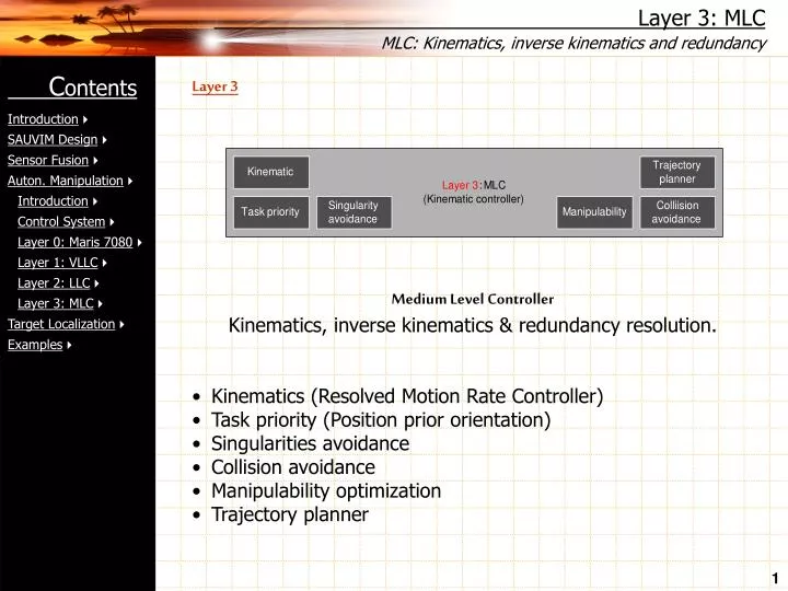
1. Contents • Introduction • SAUVIM Design • Sensor Fusion • Auton. Manipulation • Introduction • Control System • Layer 0: Maris 7080 • Layer 1: VLLC • Layer 2: LLC • Layer 3: MLC • Target Localization • Examples • Layer 3 • Medium Level Controller • Kinematics, inverse kinematics & redundancy resolution. • Kinematics (Resolved Motion Rate Controller) • Task priority (Position prior orientation) • Singularities avoidance • Collision avoidance • Manipulability optimization • Trajectory planner Layer 3: MLC MLC: Kinematics, inverse kinematics and redundancy 1

2. Contents • Introduction • SAUVIM Design • Sensor Fusion • Auton. Manipulation • Introduction • Control System • Layer 0: Maris 7080 • Layer 1: VLLC • Layer 2: LLC • Layer 3: MLC • Target Localization • Examples RMRC: Overview Resolved Motion Rate Control (RMRC) is a local method for solving inverse kinematics problems. It uses the Jacobian J of the forward kinematics to describe a change in the end-effector position as: This equation can be solved for using the Moore-Penrose pseudoinverse: Theoretical analysis Resolved Motion Rate Control 2

3. Contents • Introduction • SAUVIM Design • Sensor Fusion • Auton. Manipulation • Introduction • Control System • Layer 0: Maris 7080 • Layer 1: VLLC • Layer 2: LLC • Layer 3: MLC • Target Localization • Examples Task priority Nakamura introduced the inverse kinematics taking into account of the priority of the subtasks: Theoretical analysis Task Priority • Kinematic singularities: loss of rank of and . • Algorithmic singularities: loss of rank of with and J2 of full rank. 3

4. Contents • Introduction • SAUVIM Design • Sensor Fusion • Auton. Manipulation • Introduction • Control System • Layer 0: Maris 7080 • Layer 1: VLLC • Layer 2: LLC • Layer 3: MLC • Target Localization • Examples • In the neighbor of singular points a small change in r requires an enormous change in q, which is non-practically feasible in real manipulators and also dangerous for the structure. • Classical solutions: • Damped least-squares method (Wampler). It consists in adding a regularization term: Theoretical analysis • Problems: • Loss of performance and an increased tracking error. • Alternatives: • Variable damping factor [Nakamura] • Addition of the damping parameter only to the lowest singular values [Chiaverini]. The singularities handling problem 4

5. Contents • Introduction • SAUVIM Design • Sensor Fusion • Auton. Manipulation • Introduction • Control System • Layer 0: Maris 7080 • Layer 1: VLLC • Layer 2: LLC • Layer 3: MLC • Target Localization • Examples • Our alternative: • Using the manipulability measure as a distance criteria to avoid singularities, the proposed approach consists in a method for limiting its minimum value. • The performance is then simply affected by the choice of the lower limit. • Based on a real-time evaluation of the measure of manipulability, this method does not require a preliminary knowledge of the singular configurations. Theoretical analysis The singularities handling problem 5

6. Contents • Introduction • SAUVIM Design • Sensor Fusion • Auton. Manipulation • Introduction • Control System • Layer 0: Maris 7080 • Layer 1: VLLC • Layer 2: LLC • Layer 3: MLC • Target Localization • Examples Distance criteria: Measure of manipulability Yoshikawa (1984) proposed a continuous measure that can be regarded as a distance from singularity points (Measure of Manipulability): Theoretical analysis mom is exactly the product of the singular values of J. Advantage: its derivative with respect to the joint configuration vector q is continuous: Measure of manipulability 6

7. Contents • Introduction • SAUVIM Design • Sensor Fusion • Auton. Manipulation • Introduction • Control System • Layer 0: Maris 7080 • Layer 1: VLLC • Layer 2: LLC • Layer 3: MLC • Target Localization • Examples Task reconstruction The basic idea in task reconstruction is to circumscribe singularities by moving, when approaching to them, on a hyper-surfaces where the measure of manipulability is constants. Conceptual diagram: Theoretical analysis Task reconstruction 7

8. Contents • Introduction • SAUVIM Design • Sensor Fusion • Auton. Manipulation • Introduction • Control System • Layer 0: Maris 7080 • Layer 1: VLLC • Layer 2: LLC • Layer 3: MLC • Target Localization • Examples Our goal: In the inverse kinematics taking into account of the priority of the subtasks: Theoretical analysis Algorithm Overview The goal is to avoid both J1 and J2c becoming singular or, equivalently: 8

9. Contents • Introduction • SAUVIM Design • Sensor Fusion • Auton. Manipulation • Introduction • Control System • Layer 0: Maris 7080 • Layer 1: VLLC • Layer 2: LLC • Layer 3: MLC • Target Localization • Examples The previous criteria is also shown to be consistent with the following: Meaning: algorithmic and kinematic singularities in the inverse kinematics taking account of the priority of the subtasks will not occur when the jacobianJ of the corresponding task-space augmentation approach: is not singular. Theoretical analysis Algorithm Overview 9

10. Contents • Introduction • SAUVIM Design • Sensor Fusion • Auton. Manipulation • Introduction • Control System • Layer 0: Maris 7080 • Layer 1: VLLC • Layer 2: LLC • Layer 3: MLC • Target Localization • Examples Solution: If mom(J) is smaller than a predefined threshold m, our goal is to have: In order to realize the above condition for arbitrary dr1, firstly, we can act only a secondary (lowest priority) task correction by adding a correction term dr2c to dr2 in order to compensate the decreasing of mom(J): Theoretical analysis Algorithm Overview 10

11. Contents • Introduction • SAUVIM Design • Sensor Fusion • Auton. Manipulation • Introduction • Control System • Layer 0: Maris 7080 • Layer 1: VLLC • Layer 2: LLC • Layer 3: MLC • Target Localization • Examples Because the solution for the secondary task correction does not always exist, in order to ensure a complete singularities avoidance we must apply the task projection procedure after acting the secondary task correction: Theoretical analysis Algorithm Overview 11

12. Contents • Introduction • SAUVIM Design • Sensor Fusion • Auton. Manipulation • Introduction • Control System • Layer 0: Maris 7080 • Layer 1: VLLC • Layer 2: LLC • Layer 3: MLC • Target Localization • Examples • Implementation. • This method is suitable of a real-time implementation. The only computational costs added are: • Derivative of the jacobian: Layer 3: MLC • Measure of manipulability: Real-time implementation Using the Cholesky decomposition (JJT is a symmetric semi-positive definite matrix), the operation’s count is about m3/6 multiplication and subtractions, with also m+1 square roots. In our application, it takes about 0.4 ms on a 68060 Motorola CPU (50 MHz). 12

13. Contents • Introduction • SAUVIM Design • Sensor Fusion • Auton. Manipulation • Introduction • Control System • Layer 0: Maris 7080 • Layer 1: VLLC • Layer 2: LLC • Layer 3: MLC • Target Localization • Examples Control system General goal: tracking the target frame < g > by the tool frame < t >. Theory Control system 13

14. Contents • Introduction • SAUVIM Design • Sensor Fusion • Auton. Manipulation • Introduction • Control System • Layer 0: Maris 7080 • Layer 1: VLLC • Layer 2: LLC • Layer 3: MLC • Target Localization • Examples Feedback loop The objective of the control scheme is fundamentally that of making the global error asymptotically converging toward zero. Layer 3: MLC Closing the feedback loop The inputs is the target transformation matrix T*. Block Qf, translates the end-effector Cartesian velocity X* control signal into a corresponding set of seven joint velocity reference inputs. 14

15. Contents • Introduction • SAUVIM Design • Sensor Fusion • Auton. Manipulation • Introduction • Control System • Layer 0: Maris 7080 • Layer 1: VLLC • Layer 2: LLC • Layer 3: MLC • Target Localization • Examples • Application example. • The proposed approach has been experimented in the control of the underwater manipulator Maris7080 • The given task is a circle partially enclosed in the workspace. • The example uses the extended study taking account of the priority of the subtasks. • A comparison with damped least-squares pseudo-inversion (with variable damping factor) is given. •  Layer 3: MLC Application example 15

16. Contents • Introduction • SAUVIM Design • Sensor Fusion • Auton. Manipulation • Introduction • Control System • Layer 0: Maris 7080 • Layer 1: VLLC • Layer 2: LLC • Layer 3: MLC • Target Localization • Examples Layer 3: MLC Application example 16

17. Contents • Introduction • SAUVIM Design • Sensor Fusion • Auton. Manipulation • Introduction • Control System • Layer 0: Maris 7080 • Layer 1: VLLC • Layer 2: LLC • Layer 3: MLC • Target Localization • Examples Experimental results with the Task Projection method. Layer 3: MLC Results 17

18. Contents • Introduction • SAUVIM Design • Sensor Fusion • Auton. Manipulation • Introduction • Control System • Layer 0: Maris 7080 • Layer 1: VLLC • Layer 2: LLC • Layer 3: MLC • Target Localization • Examples Experimental results with the variable damping factor method (Nakamura) Layer 3: MLC Results 18

19. Contents • Introduction • SAUVIM Design • Sensor Fusion • Auton. Manipulation • Introduction • Control System • Layer 0: Maris 7080 • Layer 1: VLLC • Layer 2: LLC • Layer 3: MLC • Target Localization • Examples • Results. • The manipulator tries to follow the path, giving the highest priority to the position when running far the highest priority to the position when running far from a singular configuration. • Instead, when approaching to the boundary of the workspace, both the first (position) and second (orientation) manipulation variable tasks are performed with an error necessary to keep the measure of manipulability equal to the lower limit m=0.05 • Notice that it is possible to regard the proposed method as a kind of dynamic priority-changing algorithm. When the measure of manipulability of the given task approaching to zero, the highest priority is given to the distance form singularity. Layer 3: MLC Results 19

20. Contents • Introduction • SAUVIM Design • Sensor Fusion • Auton. Manipulation • Introduction • Control System • Layer 0: Maris 7080 • Layer 1: VLLC • Layer 2: LLC • Layer 3: MLC • Target Localization • Examples • Collision avoidance • With a different choice of the index function, the above approach has been proved valid to avoid obstacle collisions • The new index function is the minimum distance between the arm and the obstacle, computed simplifying each solid with a bounding box Layer 3: MLC Collision avoidance 20

21. Contents • Introduction • SAUVIM Design • Sensor Fusion • Auton. Manipulation • Introduction • Control System • Layer 0: Maris 7080 • Layer 1: VLLC • Layer 2: LLC • Layer 3: MLC • Target Localization • Examples Layer 3: MLC Collision avoidance 21

22. Contents • Introduction • SAUVIM Design • Sensor Fusion • Auton. Manipulation • Introduction • Control System • Layer 0: Maris 7080 • Layer 1: VLLC • Layer 2: LLC • Layer 3: MLC • Target Localization • Examples • Joint limit avoidance • Another index suitable of use with the precedent method is a potential function of the joint position, taking large values when the joints are far from their limits: Layer 3: MLC Joint limit avoidance 22

23. Contents • Introduction • SAUVIM Design • Sensor Fusion • Auton. Manipulation • Introduction • Control System • Layer 0: Maris 7080 • Layer 1: VLLC • Layer 2: LLC • Layer 3: MLC • Target Localization • Examples • Local maximization of manipulability • We used the redundancy in order to maximize the manipulability. This may help to keep the manipulator as far as possible from singularity configurations: Layer 3: MLC Local maximization of manipulability 23

24. Contents • Introduction • SAUVIM Design • Sensor Fusion • Auton. Manipulation • Introduction • Control System • Layer 0: Maris 7080 • Layer 1: VLLC • Layer 2: LLC • Layer 3: MLC • Target Localization • Examples Trajectory Generator (for parametric curves) It provides a smooth reference in order to track continuously from a generalized task configuration (position and orientation) to another. 1-dimensional example: Layer 3: MLC Trajectory Planner Input data are x0, xf, V0, VM, Kv and t0. 24

25. Contents • Introduction • SAUVIM Design • Sensor Fusion • Auton. Manipulation • Introduction • Control System • Layer 0: Maris 7080 • Layer 1: VLLC • Layer 2: LLC • Layer 3: MLC • Target Localization • Examples Trajectory generator example: trapezoidal case. Layer 3: MLC Trajectory generator 25

26. End of presentation

27. [Template] SD0